REMOTE SENSING OF EVAPOTRANSPIRATION FOR WATER RESOURCES MANAGEMENT

REMOTE SENSING OF EVAPOTRANSPIRATION FOR WATER RESOURCES MANAGEMENT BASIC PRINCIPLES Ayse Kilic, University of Nebraska-Lincoln Contributing Authors: Baburao Kamble (UNL), Ian Ratcliffe (UNL), Richard Allen (UI) University of Nebraska-Lincoln GIS in Water Resources Lecture, 2014

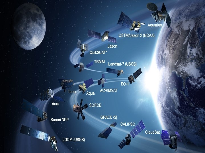
Each Landsat swath is 160 km wide Sochi Russia • Landsat is a “Polar Orbiter” in a “sun synchronous” orbit (~11: 00 am). • Landsat orbits the poles every 90 minutes. • We only get a ‘new’ image each 16 days for each spot on Earth.

Recent Landsats • Landsat 8 • Launched February 11, 2013 • 30 m pixel size for short-wave data • 100 m pixel size for thermal data • Revisit each 16 days • Landsat 7 • Launched February 1999 • 30 m pixel size for short-wave data • 60 m pixel size for thermal data • Revisit each 16 days, 8 days after Landsat 8 • Landsat 5 • Launched 1984 ended 2012 • 30 m pixel size for short-wave data • 120 m pixel size for thermal data • Revisit each 16 days • Landsat 5 retired in 2012 (worn out), replaced by L 8

What is Evapotranspiration? Soil evaporation plus leaf transpiration ET converts liquid water to vapor ET consumes water from soil that must be replaced by rainfall or irrigation ET from irrigation water is 90% of world-wide water consumption

Surface Temperature (8/29/2002) Western Nebraska Temperature (°K) Scottsbluff There is much information in Surface Temperature. There is a huge amount of surface cooling by evaporation

Some first processing of Landsat 8 images into Evapotranspiration from 800 m diameter fields in Nebraska, USA Landsat 8 – 7/12/2013 False Color Composite Bands 5/4/3 METRIC ETr. F – 7/12/2013

Landsat 8 -- Coastal area of Ventura, CA -- March 22, 2013 short-wave bands 6, 5, 4 Relative ET produced by METRIC following ‘sharpening’ of thermal data Relative ET produced by METRIC

What do we use Evapotranspiration maps for? • Better understanding of behavior of water consumption; timing. How it varies with vegetation type. • Better water balances for hydrologic studies • Ability for improved water management • Ability for improved crop production • Knowledge of water consumption by crop • Improved crop coefficient curves • Reduction of Drainage and Salinity problems • Improvement in old irrigation projects Irrigated fields in Nebraska

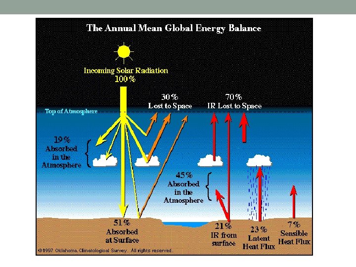
How do we determine ET from energy balance ET is calculated as a “residual” of the energy balance. This requires both short-wave and thermal imagery. • METRIC (Mapping Evapo. Transpiration with high Resolution and Internalized Calibration) • Net radiation from the sun is split into heating the air (H), heating the ground (G), or evaporating water (ET) Rn Rn= Net Radiation H ET H= Sensible Heat Flux G= Ground Heat Flux ET= Latent Heat Flux ET = R - G - H n G The energy balance includes all major sources (Rn) and consumers (ET, G, H) of energy

Rs, and Rl are shortwave and long wave radiation, respectively. The arrows show the direction of energy flow (incoming-downward; outgoing-upward). α is albedo (0 to 1) which is reflectance from the surface. ε is emissivity term (0 to 1) which is the ability to emit long wave radiation. Black body is perfect emitter ( close to 1) whereas a grey body has emissivity less than 1.

What happens to Solar Radiation in the Atmosphere H 2 O, O 2, O 3, N 2 O Indirect H 2 O, O 2, O 3, N 2 O Direct Solar (Absorbed)

Longwave (Infrared) Radiation in the Atmosphere 4 H 2 O, CO 2, CH 4, CFC’s

What we want: At Surface Reflectance ρs, b What satellite gives us: TOA Reflectance ρt, b TOA: Top of atmosphere ρt, b at-satellite reflectance for band “b” ρa, b “path” reflectance for band “b” that comes from molecules in the atmosphere τin, b and τout, b are narrowband transmittances for incoming solar radiation and for surface reflected shortwave radiation

Incoming Transmissivity (ability to transport light) C 1 -C 5 Pair W Kt qh = Generalized Coefficients fitted to MODTRAN and SMARTS 2 models = mean atmospheric pressure, k. Pa (= f(elevation)) = precipitable water in atmosphere (= f(near surface vapor pressure from weather station)) = turbidity (clearness) coefficient (default = 1. 0) = solar angle from nadir of horizontal surface Eq. has similar form to broadband t equation of FAO-56, ASCE-EWRI

Outgoing Transmissivity C 1 -C 5 Pair W Kt qh = Generalized Coefficients fitted to MODTRAN model = mean atmospheric pressure, k. Pa (= f(elevation)) = precipitable water in atmosphere (= f(near surface vapor pressure from weather station)) = turbidity (clearness) coefficient (default = 1. 0) = satellite angle from nadir of horizontal surface (0 for Landsat)

TRANSMISSIVITY (FUNCTION OF WAVELENGTH)

Broadband Surface Albedo (Bulk Reflectance) Wb = weighting coefficient that considers fraction of all potential solar energy at the surface over range represented by specific band. (Wb’s sum to 1. 0) Range for W 5 0 0. 4 0. 6 0. 8 Band: 1 2 3 4 1. 2 1. 6 5 2. 0 2. 4 Wavelength in Microns 7 weighting coefficients by Allen et al. 2006 0. 103

Vegetation Indices used to estimate the amount of vegetation on the surface which is then used to estimate aerodynamic roughness and thermal emissivity NDVI = (r 4 - r 3) / (r 4 + r 3) NDWI = (r 5 - r 2) / (r 5 + r 2) (Normalized Difference VI) (Normalized Difference Water Index) SAVI = (1 + L) (r 4 - r 3) / (L + r 4 + r 3) (Soil Adjusted VI) For Southern Idaho: L = 0. 1 SAVIID = 1. 1(r 4 - r 3) / (0. 1 + r 4 + r 3) Leaf Area Index (LAI): LAI = 11 SAVI 3 We limit LAI 6. 0 r is usually calculated at top of atmosphere

Warning!! NDVI = (r 4 - r 3) / (r 4 + r 3) (Normalized Difference VI) • Please Note! that NDVI (and SAVI) are calculated using reflectances and not digital numbers and not radiances. The variables in the equations must be ‘normalized’ reflectances, by definition. Many novices and nonthinkers commonly compute NDVI using DN or radiance. DN is improper because its scale can change over time. In addition, both DN and radiance magnitudes will change with time of year as the sun angle changes. • DN also changes with time of day. Reflectance is much more constant and consistent. One can use surface reflectance or top-of-atmosphere reflectance in the calculations. Results are usually similar since atmospheric attenuation is similar for both bands 3 and 4. • We choose to use top-of-atmosphere in METRIC NDVI to be consistent with many other uses. However, using surface reflectance is probably slightly more consistent. • Note also that NDVI computed from different satellite systems like MODIS will not be the same as from Landsat because of differences in band widths and centers.

Area just south of Albuquerque along Middle Rio Grande, New Mexico false color NDVI LAI

• Surface Emissivity • Surface Temperature

Surface Temperature (Ts) (Planck’s Law) NB is the emissivity for the narrow band Landsat thermal band (10. 45 -12. 42 μm wavelengths on Landsat 5, 10. 31 -12. 36 μm wavelengths on Landsat 7, 10. 5 – 11. 2 μm wavelengths for band 10 on Landsat 8) K 1 and K 2 are constants Rc is thermal radiance emitted from the surface in the narrow band, W/(m 2 sr μm) Ts is surface temperature in K K 1 and K 2 vary from image date to image date on Landsat 8. Therefore, you must read them from the Landsat header file that comes with the images.

Surface Emissivity NB = 0. 97 + 0. 0033 LAI; for LAI < 3 NB = 0. 98 when LAI 3 · For water; NDVI < 0 and a < 0. 47, NB = 0. 99 · For snow; NDVI < 0 and a 0. 47, NB = 0. 99 Note that some bare rock may have emissivity as low at 0. 90. The user can consult various emissivity libraries or measure.

Thermal Radiance from the Surface (Rc) Rp is the path radiance in the Landsat thermal (narrow) band that comes from molecules in the atmosphere Rsky is the narrow band thermal radiation emitted downward by a clear sky atmosphere (units are W/(m 2 sr μm) ) (we consider the 1 - e. NB component that reflects from the surface) For low aerosol conditions Rp=0. 91, transmissivity τNB=0. 866 and Rsky=1. 32, based on comparisons with MODTRAN in southern Idaho (Allen et al. 2007). LT is the radiance calculated from the digital number for thermal band.

Surface Temperature

Surface Temperature Image Red – hot (500 C) Blue – cold (200 C)

Surface Temperature Image Pathfinder-Seminoe Reservoirs, WY

Surface Energy Budget Equation Rn = G + H + ET = Rn – G – H Rn H ET G

Sensible Heat Flux is an Aerodynamic Process

Sensible Heat Flux (H) – SEBAL and METRIC H = (r × cp × d. T) / Advantage: d. T is inverse calibrated (simulated) (free of Trad vs. Taero and free of Tair) Advantage: d. T and rah ‘float’ above the surface and are ‘free’ of rah zoh and some limitations of a single source approach d. T = “floating” near surface temperature difference (K) rah = the aerodynamic resistance from z 1 to z 2 d. T z 1 u = friction velocity * k = von karmon constant (0. 41) rah H

We use electric analog to represent the heat flow (Ohm’s Law)

Near Surface Temperature Difference (d. T) • To compute the sensible heat flux (H), define near surface temperature difference (d. T) for each pixel d. T = Tnear surface – Tair d. T = Tz 1 – Tz 2 • Tair is unknown z 2 d. T rah. H z 1 • SEBAL and METRICtm assume a linear relationship between Ts and d. T: d. T = b + a. Ts

Soil Heat Flux (G) • Current G functions : LAI ≥ 0. 5 LAI < 0. 5 G = f(H) is after suggestion of Stull (1988) and development of Allen (2010, memo).

Surface Energy Balance Rn = ET + H + G ET = (Rn - H – G)/ ETr. F = ET/ETr • is Latent heat of vaporization (2. 45 MJ per Kilogram). converts ET from Energy unit (W/m 2) to an equivalent depth of water (mm) • ETr. F is fraction of reference ET and generally ranges from 0 to 1. 0. • ETr. F value of 1. 0 means that the fraction of reference ET is 1. 0, so that the ET for that pixel equals the reference ET value. • ETr is the reference ET, which is the “tall” or alfalfa reference ET that is usually calculated using the ASCE Penman-Monteith equation (ASCE 2005).

Example Applications of METRIC -Nebraska q Objective: Manage depletions to the Ogalla Aquifer. ET from irrigation extracts substantial amounts of water from the aquifer and lowers the levels. q Nebraska state law- Recognized that surface and ground water must be managed together for sustainability of water resources. q Irrigators have to reduce ground water depletion to long term sustainable levels. q Central Platte Natural Resources District (NRD) has adopted the use of Landsat based ET

Central Nebraska Irrigation District (CPNRD) – 2007 Monthly ET Central Platte Natural Resource District

Variation in ET among years (Month of July) 2011 2007 1997

Accuracy of ET maps Monthly ET estimates from METRIC were averaged over about 20 fields. Monthly ET estimates were similar to measured ET. -- Bowen Ratio energy Balance System (BRBS) data by Dr. Suat Irmak, BSE

California Imperial Valley ~15% of traditional water supply to agriculture now flows to San Diego/ Los Angeles USA ET maps help determine impacts of the water transfers on agriculture and on the Salton Sea. Mexico Graphic courtesy of R. Trezza, 2008

Montana Landsat ET has improved stream flows for endangered fisheries and to protect native American water rights 2011 ET Workshop – Boise, Idaho Graphic courtesy of J. Kjaersgaard, 2009

Montana/Wyoming • US Supreme Court – Montana v. Wyoming, No. 137, Original • --METRIC ET maps were introduced to the US Supreme Court in November 2013 to document how much irrigation water the State of Wyoming consumes from the Yellowstone River System ET Graphic courtesy of C. Kelly, 2012

ETr. F Comparison Between Landsat 8 and Landsat 7 1. 20 R 2 = 0. 9933 1. 00 Landsat 7 0. 80 ETr. F is the ‘relative’ ET rate (fraction of reference ET) 0. 60 0. 40 0. 20 0. 00 0. 20 0. 40 0. 60 Landsat 8 0. 80 1. 00 1. 20 Computations by Babu Kamble, Ian Ratcliffe, Ricardo Trezza

Reference Evapotranspiration-Google Reference Evapotranspiration represents potential ET rate when surface is covered with vegetation Daily Reference Evapotranspiration for the Entire United States 1951 – 2012 at 12 km grid Based on Grid. MET (Bias-Corrected NLDAS Data by J. Abatzoglou)

Reference Evapotranspiration-Google Earth Engine