Reminder Elements of an HMM An HMM is

Reminder

Elements of an HMM An HMM is characterized by the following: 1) N, the number of states in the model. 2) M, the number of distinct observation symbols per state. 3) the state transition probability distribution where 4) the observation symbol probability distribution in state qj, , where bj(k) is the probability that the k-th observation symbol pops up at time t, given that the model is in state Ej. 5) the initial state distribution

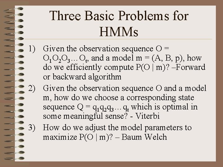
Three Basic Problems for HMMs 1) Given the observation sequence O = O 1 O 2 O 3…Ot, and a model m = (A, B, p), how do we efficiently compute P(O | m)? –Forward or backward algorithm 2) Given the observation sequence O and a model m, how do we choose a corresponding state sequence Q = q 1 q 2 q 3…qt which is optimal in some meaningful sense? - Viterbi 3) How do we adjust the model parameters to maximize P(O | m)? – Baum Welch

HMM Applications Multiple Sequence alignment Protein families and motifs Gene Finding

Multiple Sequence Alignment -MSA

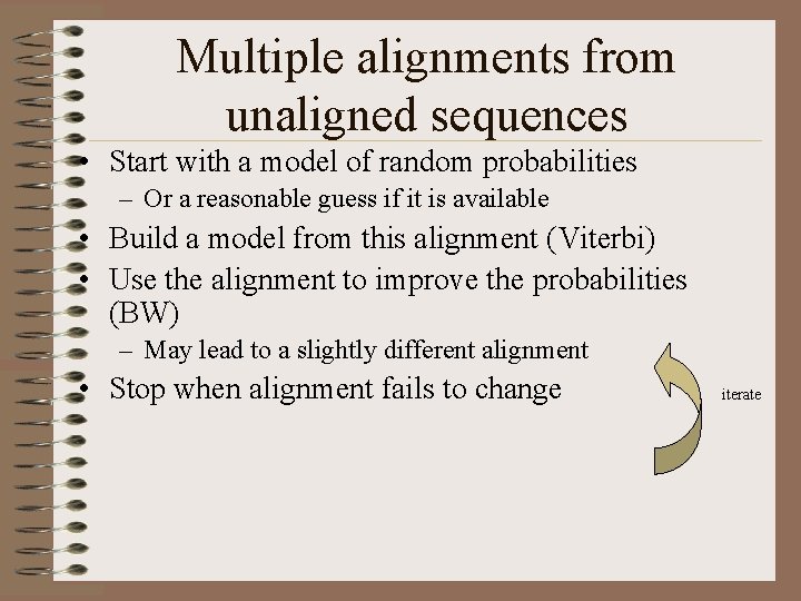
Multiple alignments from unaligned sequences • Start with a model of random probabilities – Or a reasonable guess if it is available • Build a model from this alignment (Viterbi) • Use the alignment to improve the probabilities (BW) – May lead to a slightly different alignment • Stop when alignment fails to change iterate

Some preliminary remarks • Sequence alignment is useful for discovering functional, structural, and evolutionary information in biological research. • Different metrics (or notions of distance) could be defined to compare sequences. • Mathematician Peter Sellers (1974) showed that if a sequence alignment is formulated in terms of distances instead of similarity, a biologically more appealing interpretation of gaps is possible. • The latter is an evolution-motivated definition, relying on the concept of ancestry.

Multiple Sequence Alignment • The MSA of a set of sequences may be viewed as an evolutionary history of the sequences. • HMMs often provide a MSA as good as, if not better than, other methods. • No sequence ordering is required. • Insertion/deletion penalties are not needed. • The aligned sequences are used as the training data, to train the parameters of the model. • For each sequence, the Viterbi algorithm is then used to determine a path most likely to have produced that sequence. • This in turn can be used to realign the sequences

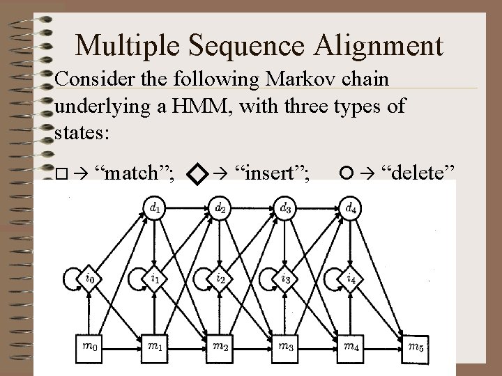
Multiple Sequence Alignment Consider the following Markov chain underlying a HMM, with three types of states: “match”; “insert”; “delete”

Modeling Protein Families • The states of our HMM will be divided into match states, insert states and delete states. • It is useful to include an initial state and a final one, and we assume that no match or delete state is visited more than once. • The alphabet M consists of twenty amino acids together with one dummy symbol representing “delete”. Delete states output only. • Each insert and match state has its own distribution over the 20 amino acids, and does not emit the symbol .

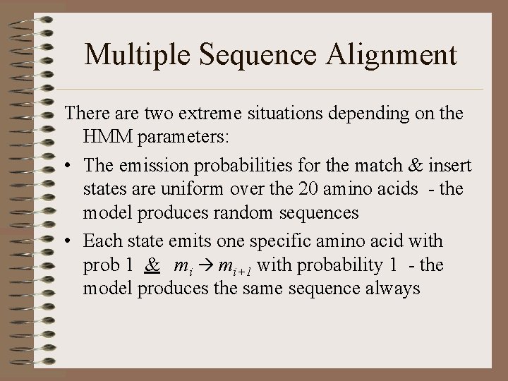
Multiple Sequence Alignment There are two extreme situations depending on the HMM parameters: • The emission probabilities for the match & insert states are uniform over the 20 amino acids - the model produces random sequences • Each state emits one specific amino acid with prob 1 & mi mi+1 with probability 1 - the model produces the same sequence always

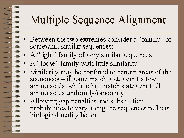
Multiple Sequence Alignment • Between the two extremes consider a “family” of somewhat similar sequences: • A “tight” family of very similar sequences • A “loose” family with little similarity • Similarity may be confined to certain areas of the sequences – if some match states emit a few amino acids, while other match states emit all amino acids uniformly/randomly • Allowing gap penalties and substitution probabilities to vary along the sequences reflects biological reality better.

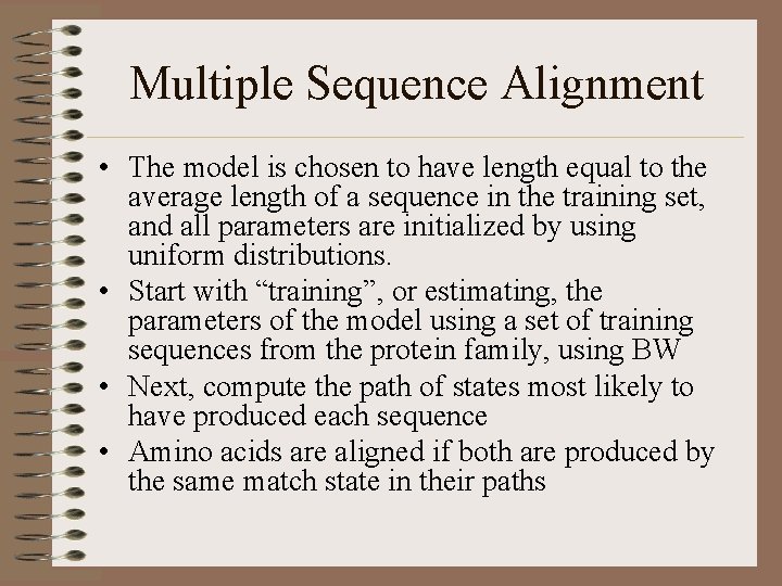
Multiple Sequence Alignment • The model is chosen to have length equal to the average length of a sequence in the training set, and all parameters are initialized by using uniform distributions. • Start with “training”, or estimating, the parameters of the model using a set of training sequences from the protein family, using BW • Next, compute the path of states most likely to have produced each sequence • Amino acids are aligned if both are produced by the same match state in their paths

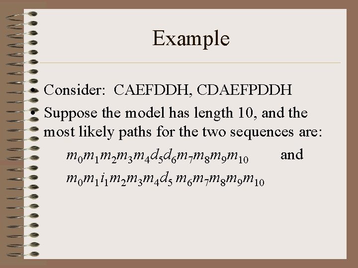
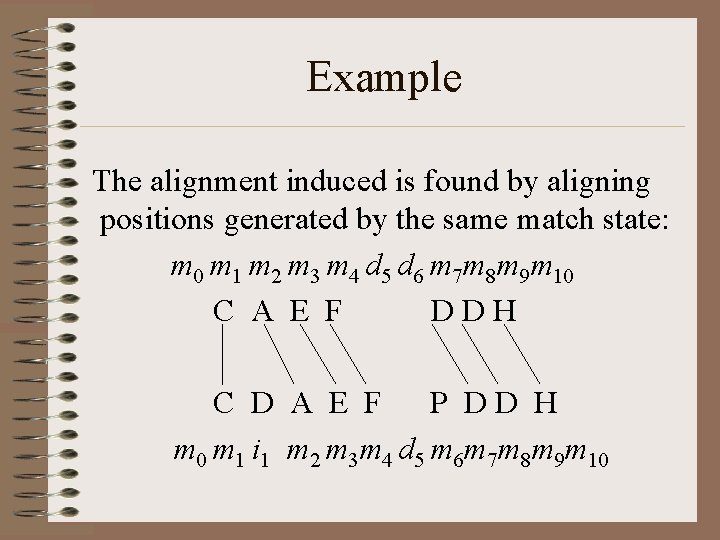
Example • Consider: CAEFDDH, CDAEFPDDH • Suppose the model has length 10, and the most likely paths for the two sequences are: m 0 m 1 m 2 m 3 m 4 d 5 d 6 m 7 m 8 m 9 m 10 and m 0 m 1 i 1 m 2 m 3 m 4 d 5 m 6 m 7 m 8 m 9 m 10

Example The alignment induced is found by aligning positions generated by the same match state: m 0 m 1 m 2 m 3 m 4 d 5 d 6 m 7 m 8 m 9 m 10 C A E F DDH C D A E F P DD H m 0 m 1 i 1 m 2 m 3 m 4 d 5 m 6 m 7 m 8 m 9 m 10

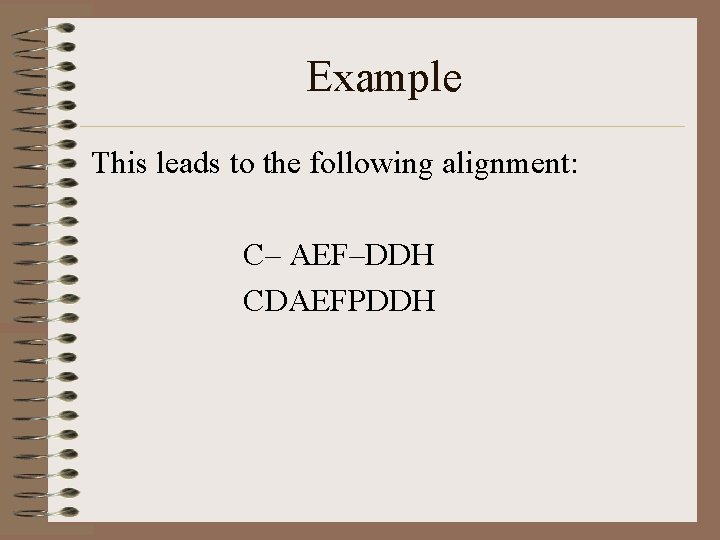
Example This leads to the following alignment: C– AEF–DDH CDAEFPDDH

Gene Finding

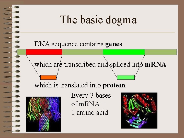
The basic dogma DNA sequence contains genes which are transcribed and spliced into m. RNA which is translated into protein. Every 3 bases of m. RNA = 1 amino acid

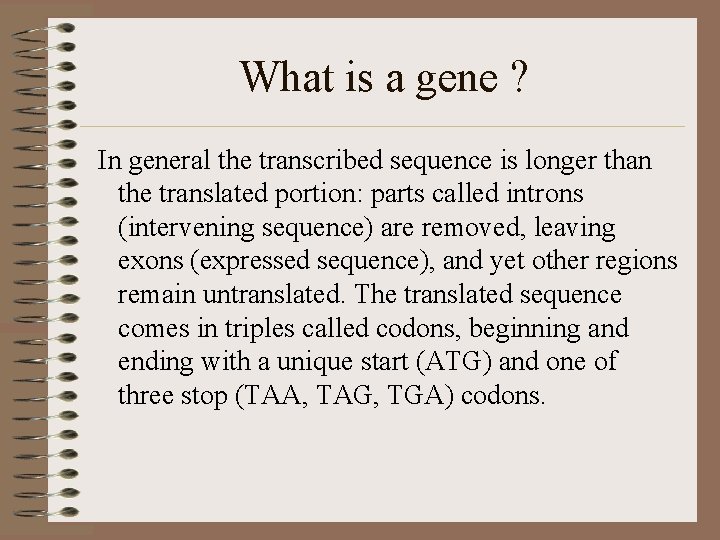
What is a gene ? In general the transcribed sequence is longer than the translated portion: parts called introns (intervening sequence) are removed, leaving exons (expressed sequence), and yet other regions remain untranslated. The translated sequence comes in triples called codons, beginning and ending with a unique start (ATG) and one of three stop (TAA, TAG, TGA) codons.

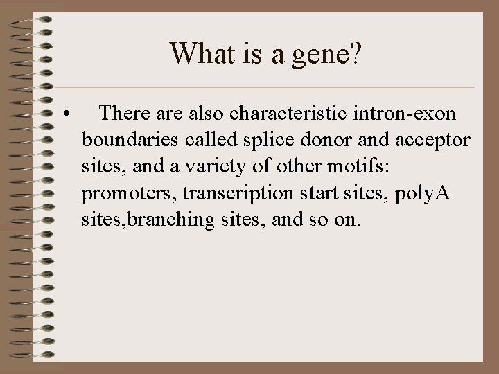
What is a gene? • There also characteristic intron-exon boundaries called splice donor and acceptor sites, and a variety of other motifs: promoters, transcription start sites, poly. A sites, branching sites, and so on.

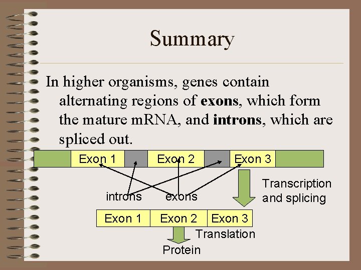
Summary In higher organisms, genes contain alternating regions of exons, which form the mature m. RNA, and introns, which are spliced out. Exon 1 introns Exon 1 Exon 2 Exon 3 exons Exon 2 Exon 3 Translation Protein Transcription and splicing

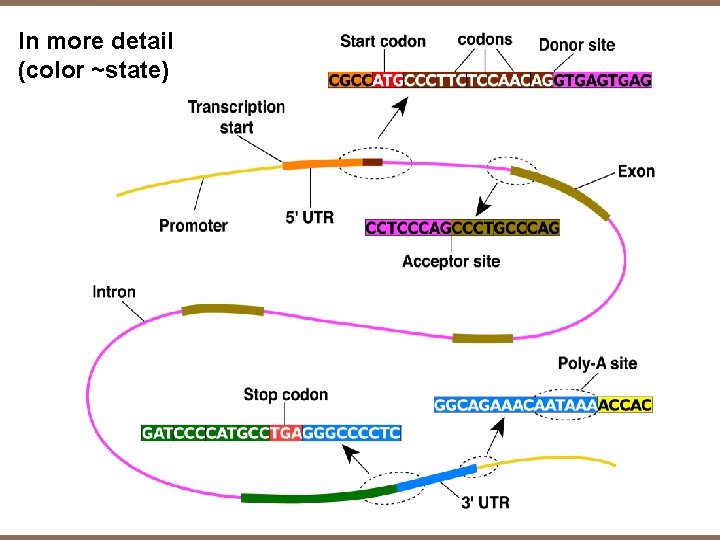
In more detail (color ~state)

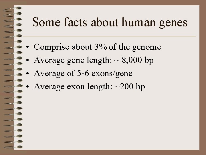
Some facts about human genes • • Comprise about 3% of the genome Average gene length: ~ 8, 000 bp Average of 5 -6 exons/gene Average exon length: ~200 bp

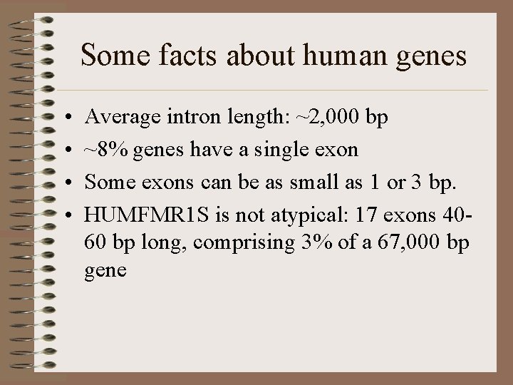
Some facts about human genes • • Average intron length: ~2, 000 bp ~8% genes have a single exon Some exons can be as small as 1 or 3 bp. HUMFMR 1 S is not atypical: 17 exons 4060 bp long, comprising 3% of a 67, 000 bp gene

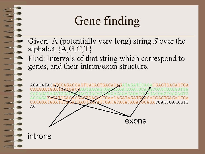
Gene finding • Given: A (potentially very long) string S over the alphabet {A, G, C, T} • Find: Intervals of that string which correspond to genes, and their intron/exon structure. ACAGATGCAGACGAGTGACACAGATAGATGCAGACGAGTGACAGTGACACAGATGCAGACGAGTGACAGTG ACCAGATGCAGACGAGTGACAGTGAACAGATGCAGACGAGTGACAGTGA CACAGATGCAGACGAGTGACACAGATGCAGACGAGTGACAGTG AC exons introns

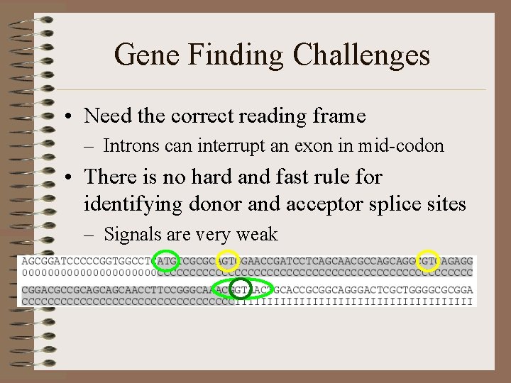
Gene Finding Challenges • Need the correct reading frame – Introns can interrupt an exon in mid-codon • There is no hard and fast rule for identifying donor and acceptor splice sites – Signals are very weak

The idea behind a GHMM genefinder • States represent standard gene features: intergenic region, exon, intron, perhaps more (promotor, 5’UTR, 3’UTR, Poly-A, . . ). • Observations embody state-dependent base composition, dependence, and signal features. • In a GHMM, duration must be included as well. Finally, reading frames and both strands must be dealt with.

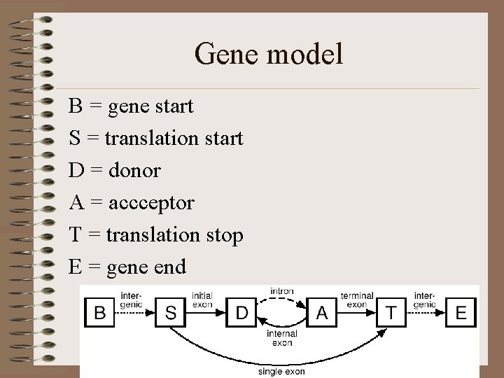
Gene model B = gene start S = translation start D = donor A = accceptor T = translation stop E = gene end

Why HMMs might be a good fit for Gene Finding • Classification: Classifying observations within a sequence • Order: A DNA sequence is a set of ordered observations • Grammar / Architecture: Our grammatical structure (and the beginnings of our architecture) is right here: • Success measure: # of complete exons correctly labeled • Training data: Available from various genome annotation projects

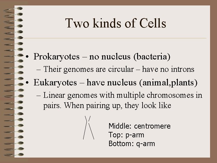
Two kinds of Cells • Prokaryotes – no nucleus (bacteria) – Their genomes are circular – have no introns • Eukaryotes – have nucleus (animal, plants) – Linear genomes with multiple chromosomes in pairs. When pairing up, they look like Middle: centromere Top: p-arm Bottom: q-arm

Prokaryotes

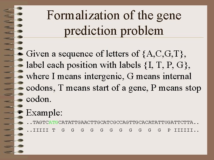
Formalization of the gene prediction problem • Given a sequence of letters of {A, C, G, T}, label each position with labels {I, T, P, G}, where I means intergenic, G means internal codons, T means start of a gene, P means stop codon. • Example: • . . TAGTCATGCATATTGAACTTGCATCGCCAGTTGCACATATTUGATTCTTA. . • . . IIIII T G G G P IIIIII. .

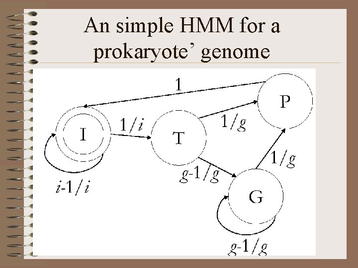
An simple HMM for a prokaryote’ genome

Problem • The output letter of the HMM at one state only depends on the state itself. However, it should also depends on the previous output letter(s). • A more complex HMM • Replace Pr(output | current_state) by Pr(output | current_state, previous_output)

Eukaryotes

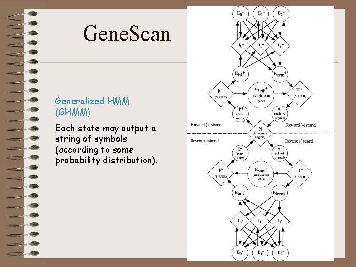
Gene. Scan Generalized HMM (GHMM) Each state may output a string of symbols (according to some probability distribution).

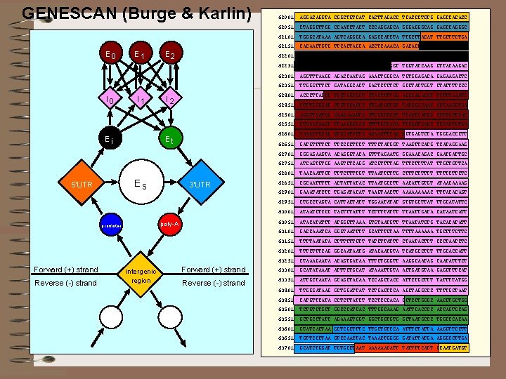
GENESCAN (Burge & Karlin) E 0 I 0 E 1 I 1 Ei Reverse (-) strand 62051 CTAGGGTTGG CCAATCTACT CCCAGGAGCA GGGAGGGCAG GAGCCAGGGC 62101 TGGGCATAAA AGTCAGGGCA GAGCCATCTA TTGCTTACAT TTGCTTCTGA 62151 CACAACTGTG TTCACTAGCA ACCTCAAACA GACACCATGG TGCACCTGAC 62201 TCCTGAGGAG AAGTCTGCCG TTACTGCCCT GTGGGGCAAG GTGAACGTGG 62251 ATGAAGTTGG TGGTGAGGCC CTGGGCAGGT TGGTATCAAG GTTACAAGAC 62301 AGGTTTAAGG AGACCAATAG AAACTGGGCA TGTGGAGACA GAGAAGACTC 62351 TTGGGTTTCT GATAGGCACT GACTCT GCCTATTGGT CTATTTTCCC 62401 ACCCTTAGGC TGCTGGTGGT CTACCCTTGG ACCCAGAGGT TCTTTGAGTC 62451 CTTTGGGGAT CTGTCCACTC CTGATGCTGT TATGGGCAAC CCTAAGGTGA 62501 AGGCTCATGG CAAGAAAGTG CTCGGTGCCT TTAGTGATGG CCTGGCTCAC 62551 CTGGACAACC TCAAGGGCAC CTTTGCCACA CTGAGC TGCACTGTGA 62601 CAAGCTGCAC GTGGATCCTG AGAACTTCAG GGTGAGTCTA TGGGACCCTT 62651 GATGTTTTCT TTCCCCTTCT TTTCTATGGT TAAGTTCATG TCATAGGAAG 62701 GGGAGAAGTA ACAGGGTACA GTTTAGAATG GGAAACAGAC GAATGATTGC 62751 ATCAGTGTGG AAGTCTCAGG ATCGTTTTAG TTTCTTTTAT TTGCTGTTCA 62801 TAACAATTGT TTTCTTTTGT TTAATTCTTG CTTTTTCTTCTC 62851 CGCAATTTTT ACTATTATAC TTAATGCCTT AACATTGTGT ATAACAAAAG 62901 GAAATATCTC TGAGATACAT TAAGTAACTT AAAAAC TTTACACAGT 62951 CTGCCTAGTA CATTACTATT TGGAATATAT GTGTGCTTAT TTGCATATTC 63001 ATAATCTCCC TACTTTATTT TCTTTTATTT TTAATTGATA CATAATCATT 63051 ATACATATTT ATGGGTTAAA GTGTAATGTT TTAATATGTG TACACATATT 63101 GACCAAATCA GGGTAATTTT GCATTTGTAA TTTTAAAAAA TGCTTTCTTC 63151 TTTTAATATA CTTTTTTGTT TATCTTATTT CTAATACTTT CCCTAATCTC 63201 TTTCAG GGCAATAATG ATACAATGTA TCATGCCTCT TTGCACCATT 63251 CTAAAGAATA ACAGTGATAA TTTCTGGGTT AAGGCAATAG CAATATTTCT Forward (+) strand 63301 GCATATAAAT ATTTCTGCAT ATAAATTGTA ACTGATGTAA GAGGTTTCAT Reverse (-) strand 63351 ATTGCTAATA GCAGCTACAA TCCAGCTACC ATTCTGCTTT TATTTTATGG 63401 TTGGGATAAG GCTGGATTAT TCTGAGTCCA AGCTAGGCCC TTTTGCTAAT 63451 CATGTTCATA CCTCTTATCT TCCTCCCACA GCTCCTGGGC AACGTGCTGG 63501 TCTGTGTGCT GGCCCATCAC TTTGGCAAAG AATTCACCCC ACCAGTGCAG 63551 GCTGCCTATC AGAAAGTGGT GGCTGGTGTG GCTAATGCCC TGGCCCACAA 63601 GTATCACTAA GCTCGCTTTC TTGCTGTCCA ATTTCTATTA AAGGTTCCTT 63651 TGTTCCCTAA GTCCAACTAC TAAACTGGGG GATATTATGA AGGGCCTTGA 63701 GCATCTGGAT TCTGCCTAAT AAAAAACATT TATTTTCATT GCAATGATGT I 2 Et 3'UTR poly-A promoter Forward (+) strand AGGACAGGTA CGGCTGTCAT CACTTAGACC TCACCCTGTG GAGCCACACC E 2 Es 5'UTR 62001 intergenic region

Gene. Scan • Currently, a popular and successful gene finder for human DNA sequences is GENSCAN (Burge et al. 1997. ) • It is based on a generalization of HMMs, called Semi hidden Markov Models. • The algorithms involved in this model are an order of magnitude more complex than for a regular HMM. • The gene-finding application requires a generalization of the Viterbi algorithm.

Gene. Scan • Burge (1997) observed that if the lengths of the long intergenic regions can be taken as having geometric distributions, and if these lengths generate sequences in a relatively iid fashion, then the algorithm can be adjusted so that practical running times can be obtained.

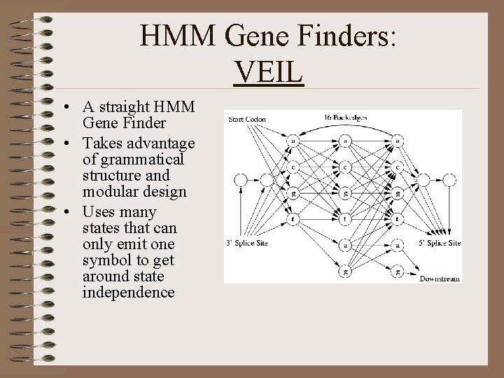
HMM Gene Finders: VEIL • A straight HMM Gene Finder • Takes advantage of grammatical structure and modular design • Uses many states that can only emit one symbol to get around state independence

Effectiveness of HMM-based finders • The best gene-finding HMM (Gen. Scan, Burge and Karlin 1997) has ~80% sensitivity and ~80% specificity at the exon level. (That is, roughly 80% of true exons are entirely correctly found, and about 80% of the predicted exons are entirely correct. )

Beyond position-specific distributions • The bases in splice sites exhibit dependence, and not simply of the nearest neighbor kind. • High-order (non-stationary) Markov models would be one option, but the number of parameters in relation to the amount of data rules them out. The class of variable length Markov models (VLMMs) deriving from early research by Rissanen prove to be valuable in this context.

Protein Famillies

Pfam • Pfam is a web-based resource maintained by the Sanger Center http: //www. sanger. ac. uk/Pfam • Pfam uses the basic theory described above to determine protein domains in a query sequence. • Suppose that a new protein is obtained for which no information is available except the raw sequence. • We wish to “annotate” this sequence.

Protein Family Classification • Pfam • large collection of multiple sequence alignments and hidden Markov models • covers many common protein domains and families – Over 73% of all known protein sequences have at least one match – 5, 193 different protein families

Pfam Family Types • family – default classification, stating members are related • domain – structural unit found in multiple protein contexts • repeat –domain that in itself is not stable, but when combined with multiple tandem repeats forms a domain or structure • motif – shorter sequence units found outside of domains

Pfam • Initial multiple alignment of seeds using a program such as Clustal • Alignment hand scrutinized and adjusted • additional sequences are added to the family by comparing the HMM against sequence databases • Resulting full alignments with additional family members may look worse than initial seed alignments