REMI Tran Sight An InDepth Look Regional Economic

REMI® Tran. Sight™: An In-Depth Look Regional Economic Models, Inc. Amherst, MA

Overview of Presentation • • • Tran. Sight REMI Policy Insight Travel Demand Models Modeling Transportation Impacts Viewing Results

Regional Economic Models, Inc. (REMI) provides… n Policy Insight: A macroeconomic forecasting model that shows the total economic, demographic and fiscal effects of policy initiatives on local regions n Tran. Sight: A model that integrates Policy Insight with transport planning and travel demand models to show the total economic, demographic, and fiscal effects of transportation infrastructure projects

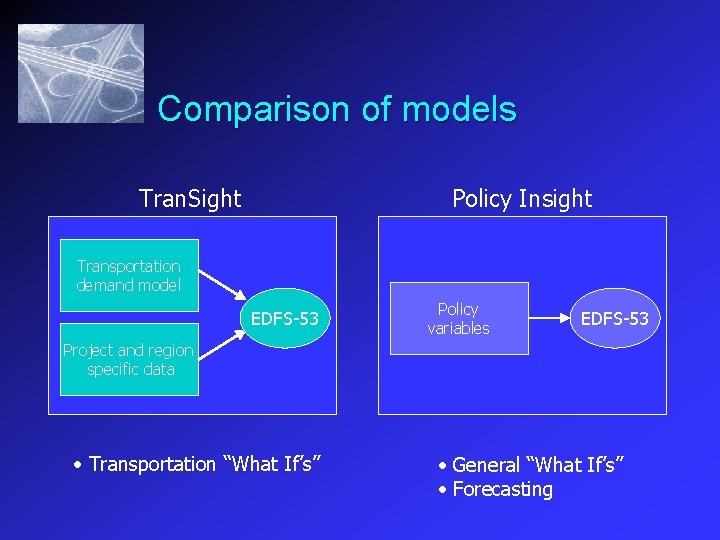
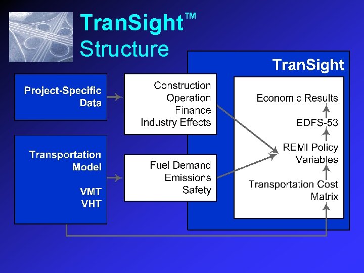
Comparison of models Tran. Sight Policy Insight Transportation demand model EDFS-53 Policy variables EDFS-53 Project and region specific data • Transportation “What If’s” • General “What If’s” • Forecasting

REMI Tran. Sight™ First and foremost, REMI Tran. Sight integrates REMI Policy Insight®—the world’s leading economic and fiscal policy analysis and simulation model—with the transport planning and travel demand models used most often by government and private sector planners.

REMI Tran. Sight™ And because REMI Policy Insight® embodies the latest research advances in economic geography, REMI Tran. Sight can show transportation planners and policy makers the total economic effects of new investments in highways, transit, and other transportation infrastructure.

REMI Tran. Sight™ In particular, REMI Tran. Sight can quantify the unique contribution transportation investments make toward creating and expanding industry clusters, some of the main drivers in diversifying and sustaining regional economic development.

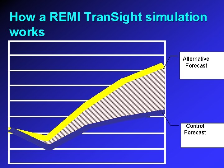
How a REMI Tran. Sight simulation works Alternative Forecast Control Forecast

Tran. Sight™ Structure

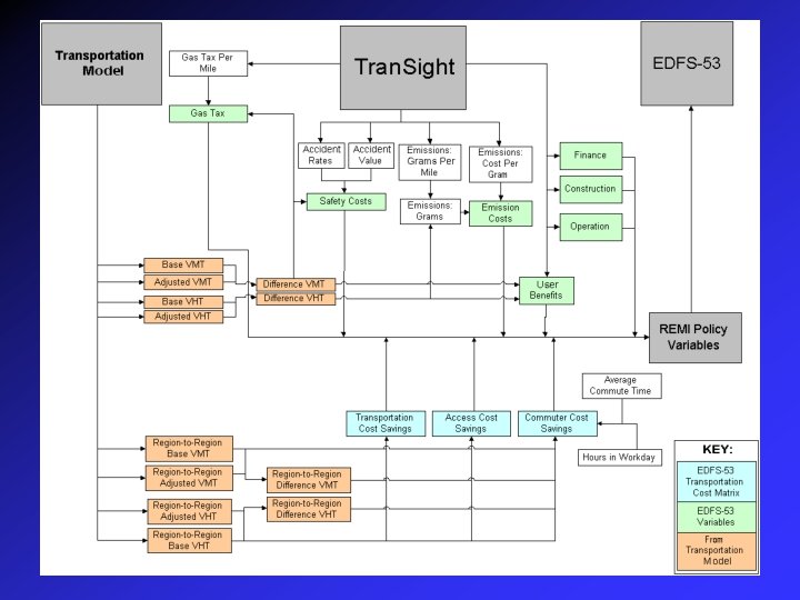
Transight™ Structure Complex

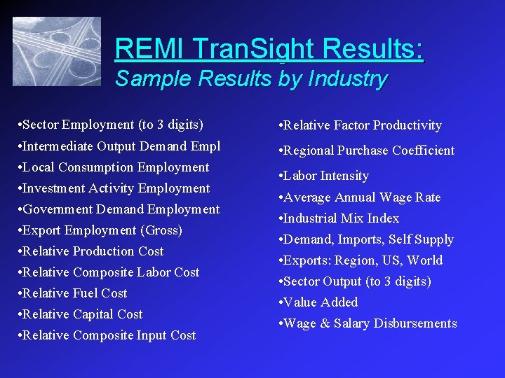
REMI Tran. Sight Results: Sample Results by Industry • Sector Employment (to 3 digits) • Relative Factor Productivity • Intermediate Output Demand Empl • Local Consumption Employment • Investment Activity Employment • Government Demand Employment • Export Employment (Gross) • Relative Production Cost • Relative Composite Labor Cost • Relative Fuel Cost • Relative Capital Cost • Relative Composite Input Cost • Regional Purchase Coefficient • Labor Intensity • Average Annual Wage Rate • Industrial Mix Index • Demand, Imports, Self Supply • Exports: Region, US, World • Sector Output (to 3 digits) • Value Added • Wage & Salary Disbursements

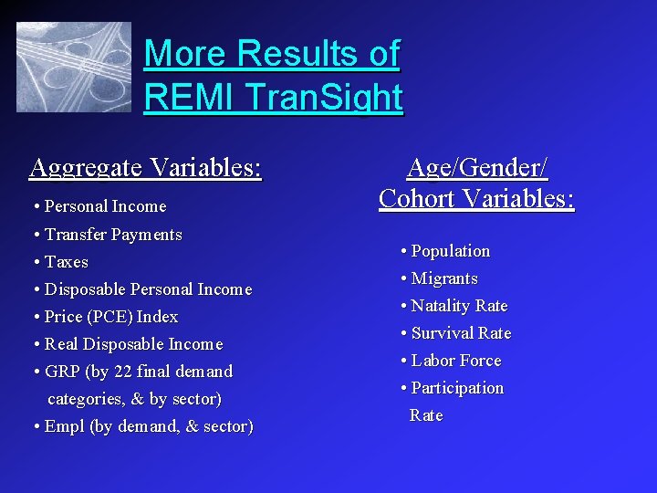
More Results of REMI Tran. Sight Aggregate Variables: • Personal Income • Transfer Payments • Taxes • Disposable Personal Income • Price (PCE) Index • Real Disposable Income • GRP (by 22 final demand categories, & by sector) • Empl (by demand, & sector) Age/Gender/ Cohort Variables: • Population • Migrants • Natality Rate • Survival Rate • Labor Force • Participation Rate

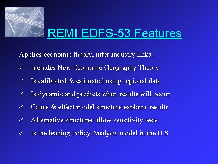
REMI EDFS-53 Features Applies economic theory, inter-industry links: ü Includes New Economic Geography Theory ü Is calibrated & estimated using regional data ü Is dynamic and predicts when results will occur ü Cause & effect model structure explains results ü Alternative structures allow sensitivity tests ü Is the leading Policy Analysis model in the U. S.

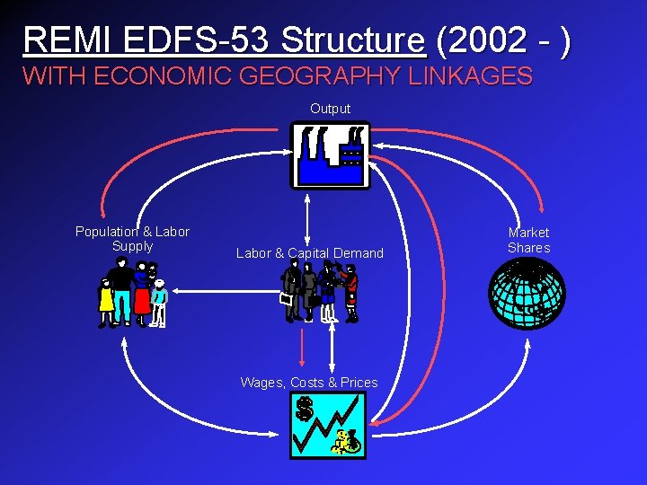
REMI EDFS-53 Structure (2002 - ) WITH ECONOMIC GEOGRAPHY LINKAGES Output Population & Labor Supply Labor & Capital Demand Wages, Costs & Prices Market Shares

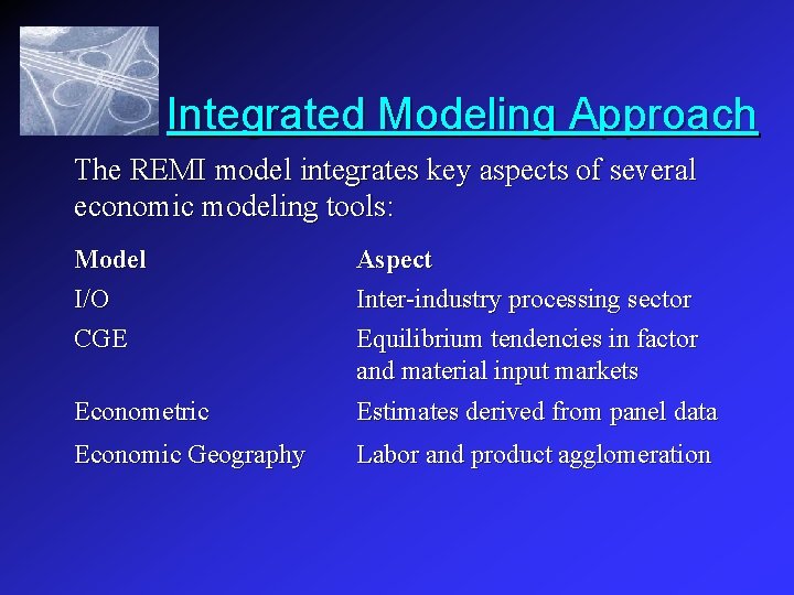
Integrated Modeling Approach The REMI model integrates key aspects of several economic modeling tools: Model I/O CGE Aspect Inter-industry processing sector Equilibrium tendencies in factor and material input markets Econometric Estimates derived from panel data Economic Geography Labor and product agglomeration

New Economic Geography n n n Based on monopolistic competition Increasing economies of scale for firms (decreasing marginal costs). Access to product varieties from different regions. Different delivered prices in the same industry due to transportation or other distance deterrence costs. Cross hauling, cluster agglomeration, and labor productivity are explained by microeconomic gains from having choice and variety.

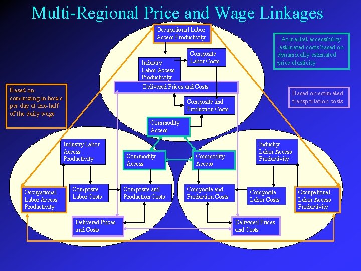
New EG Features Labor Productivity Concepts n n n Labor Access Index u Occupation & industry effects of selecting best workers Composite Labor Cost u Relative wage rate adjusted for labor access index u Includes commuter distance cost blended into wage rates Occupation Codes u Standard occupation codes (SOCs) are implemented u Better groupings with sectors for analysis & display

New EG Features Commodity Price Concepts n Delivered Price (wtd avg by sector at place of use) u u n Commodity Access Index (by sector at place of use) u u n Producer & consumer effects of better commodity choice Reflects market share changes due to composite price changes Composite Price (by sector at place of use) u n Source production cost + transport cost to place of use Production & transport costs reflect every source location Delivered price adjusted for commodity access index Production Cost (by sector at place of use) u u Includes intermediate inputs from all sectors & locations Local production cost captures intermediate input composite prices; composite labor cost; and capital and fuel costs

New EG Features Trade Flows and Market Shares n Trade Flows Treatment u n Shows trade flows from each region to each other region in the model, plus rest of US and rest of world Domestic Market Shares Display u Shows share of local demand met by regions in model

New EG Features Transportation Costs Matrix There are three components of the matrix: Commuting costs u Accessibility costs u Transportation costs u The three components respond to changes in the effective distance between regions.

Multi-Regional Price and Wage Linkages Occupational Labor Access Productivity Industry Labor Access Productivity At market accessibility estimated costs based on dynamically estimated price elasticity Composite Labor Costs Delivered Prices and Costs Based on commuting in hours per day at one-half of the daily wage Based on estimated transportation costs Composite and Production Costs Commodity Access Industry Labor Access Productivity Occupational Labor Access Productivity Composite Labor Costs Delivered Prices and Costs Commodity Access Composite and Production Costs Industry Labor Access Productivity Composite Labor Costs Delivered Prices and Costs Occupational Labor Access Productivity

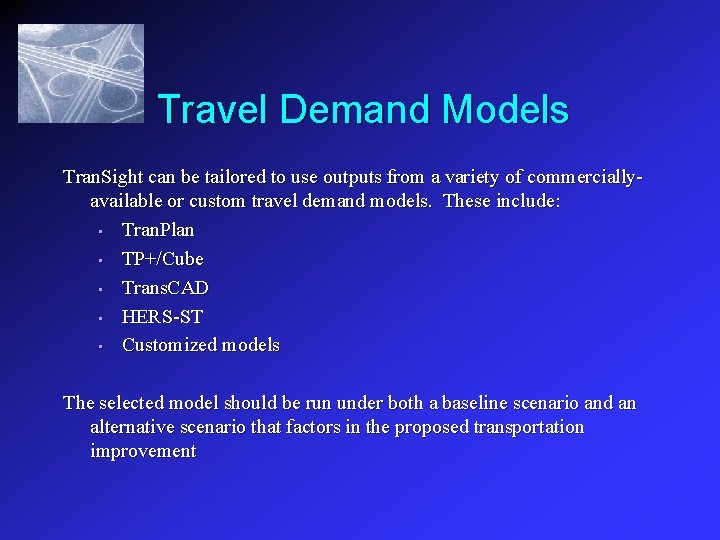
Travel Demand Models Tran. Sight can be tailored to use outputs from a variety of commerciallyavailable or custom travel demand models. These include: • Tran. Plan • TP+/Cube • Trans. CAD • HERS-ST • Customized models The selected model should be run under both a baseline scenario and an alternative scenario that factors in the proposed transportation improvement

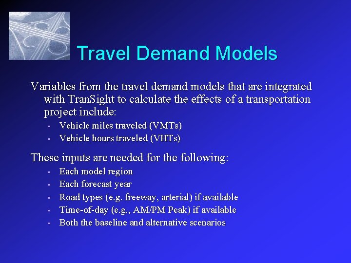
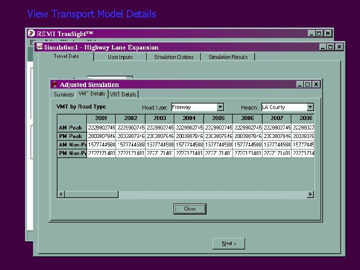
Travel Demand Models Variables from the travel demand models that are integrated with Tran. Sight to calculate the effects of a transportation project include: • • Vehicle miles traveled (VMTs) Vehicle hours traveled (VHTs) These inputs are needed for the following: • • • Each model region Each forecast year Road types (e. g. freeway, arterial) if available Time-of-day (e. g. , AM/PM Peak) if available Both the baseline and alternative scenarios

View Transport Model Details

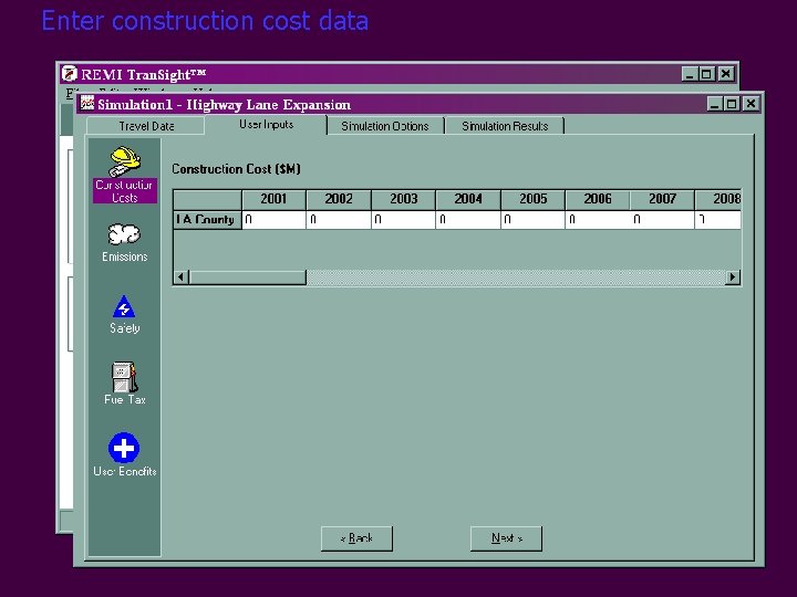
Construction and Maintenance Costs Overview: n Projected annual costs incurred by government for construction, maintenance and repair are entered by user n Project financing can be split between federal, state, and local government n Work is usually contracted out to private construction firms, which creates jobs and demand for intermediate inputs n Operation and maintenance costs more significant for public transit than roads

Construction and Maintenance Costs The EDFS-53 connection: • • Increased annual sales by the construction industry, to reflect expenses on construction and upkeep Government expenditures, apportioned to federal, state and local levels according to financing percentages

Enter construction cost data

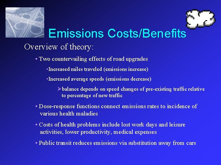
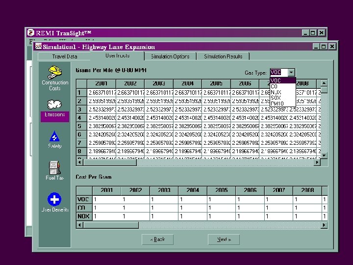
Emissions Costs/Benefits Overview of theory: • Two countervailing effects of road upgrades • Increased miles traveled (emissions increase) • Increased average speeds (emissions decrease) Øbalance depends on speed changes of pre-existing traffic relative to percentage of new traffic • Dose-response functions connect emissions rates to incidence of various health maladies • Costs of health problems include lost work days and leisure activities, lower productivity, medical expenses • Public transit reduces emissions via substitution away from cars

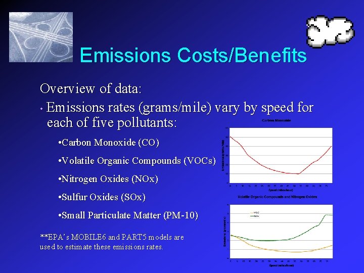
Emissions Costs/Benefits Overview of data: • Emissions rates (grams/mile) vary by speed for each of five pollutants: • Carbon Monoxide (CO) • Volatile Organic Compounds (VOCs) • Nitrogen Oxides (NOx) • Sulfur Oxides (SOx) • Small Particulate Matter (PM-10) **EPA’s MOBILE 6 and PART 5 models are used to estimate these emissions rates.

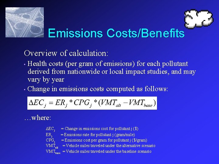
Emissions Costs/Benefits Overview of calculation: Health costs (per gram of emissions) for each pollutant derived from nationwide or local impact studies, and may vary by year • Change in emissions costs computed as follows: • …where: ECj = Change in emissions cost for pollutant j ($) ERj = Emissions rate for pollutant j (gram/mile) CPGj = Emissions cost per gram for pollutant j ($/gram) VMTalt = Vehicle miles traveled under the alternative scenario VMTbase = Vehicle miles traveled under the baseline scenario

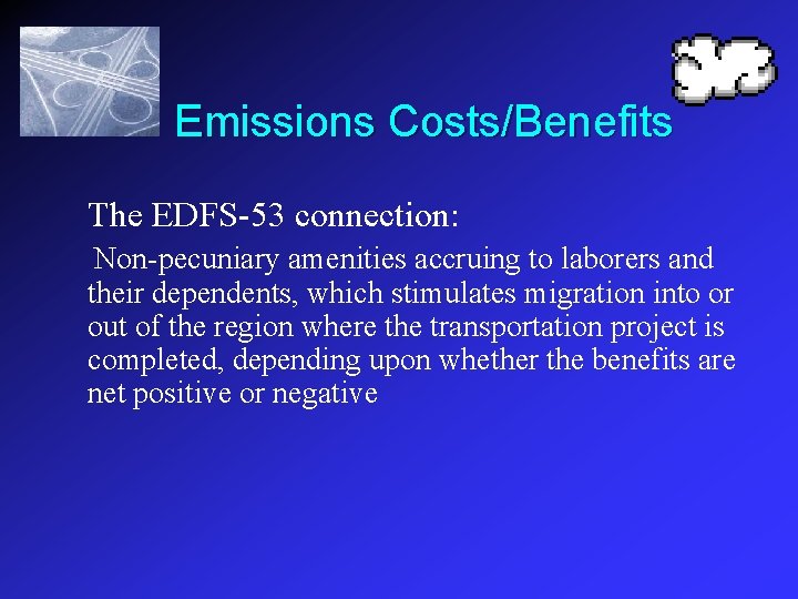
Emissions Costs/Benefits The EDFS-53 connection: Non-pecuniary amenities accruing to laborers and their dependents, which stimulates migration into or out of the region where the transportation project is completed, depending upon whether the benefits are net positive or negative

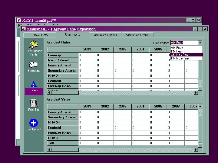
Safety Costs/Benefits Overview: n Benefits/costs of a transportation project include the following aspects u The values of injuries and lives lost* t This value may increase due to a gain in miles traveled t This value may decrease due to safety improvements u Property damage** u Delay due to automobile accidents** n May vary by year to reflect rising medical and insurance costs *Value taken from U. S. DOT estimation of the value of life (currently $3 mil/life) **Value taken from National Highway Traffic Safety Administration, The Economic Cost of Motor Vehicle Crashes 1994; Lawrence J. Blincoe, 1996

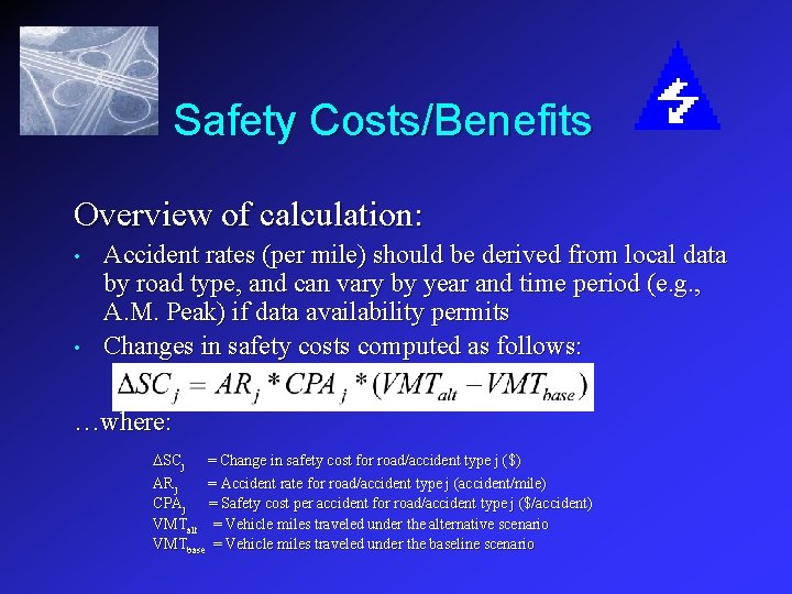
Safety Costs/Benefits Overview of calculation: • • Accident rates (per mile) should be derived from local data by road type, and can vary by year and time period (e. g. , A. M. Peak) if data availability permits Changes in safety costs computed as follows: …where: SCj = Change in safety cost for road/accident type j ($) ARj = Accident rate for road/accident type j (accident/mile) CPAj = Safety cost per accident for road/accident type j ($/accident) VMTalt = Vehicle miles traveled under the alternative scenario VMTbase = Vehicle miles traveled under the baseline scenario

Safety Costs/Benefits The EDFS-53 Connection: Non-pecuniary amenities to households, which stimulates migration into or out of the region where the transportation project is completed, depending upon whether the benefits are net positive or negative

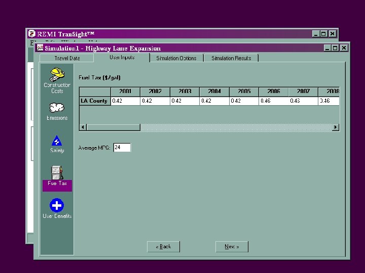
Fuel Tax Changes Overview u § Change in fuel tax revenues proportional to change in gallons consumed, which can move two ways following a road upgrade: 1) Incremental travel demand: gallons increase 2) Higher average speeds of existing traffic: gallons decrease New or expanded public transit will induce substitution away from cars; magnitude of switch will determine tax revenue change

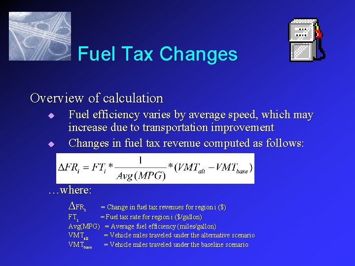
Fuel Tax Changes Overview of calculation u u Fuel efficiency varies by average speed, which may increase due to transportation improvement Changes in fuel tax revenue computed as follows: …where: FR = Change in fuel tax revenues for region i ($) FTi = Fuel tax rate for region i ($/gallon) Avg(MPG) = Average fuel efficiency (miles/gallon) VMTalt = Vehicle miles traveled under the alternative scenario VMTbase = Vehicle miles traveled under the baseline scenario i

Fuel Tax Changes The EDFS-53 Connection: The policy variable effect can be tailored to the client’s specifications: say, a change in funds available for government spending, or an adjustment to the model’s fiscal balancing mechanism

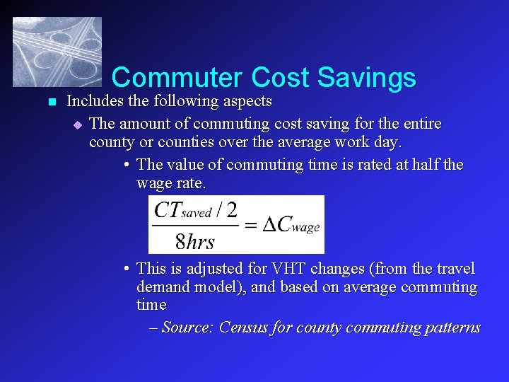
Commuter Cost Savings n Includes the following aspects u The amount of commuting cost saving for the entire county or counties over the average work day. • The value of commuting time is rated at half the wage rate. • This is adjusted for VHT changes (from the travel demand model), and based on average commuting time – Source: Census for county commuting patterns

Commuting Costs The EDFS-53 Connection: • • Commuting costs affect the effective distance in the occupational labor access productivity equation (by adjusting labor cost relative to the average wage rate), which feeds into industry labor access productivity and from there into composite wage rates This ultimately affects both the composite cost of production by industry and the relative wage rate in the economic migration equation.

Transportation Cost Savings n Includes the following aspects u The cost savings in transporting goods and services due to increase in transportation efficiency t These are calculated from changes in VMT and VHT between the alternative simulation and baseline control t Source: Travel demand model

Transportation Costs The EDFS-53 Connection: • • Transportation costs affect the effective distance in the delivered price equation for each sector (relative to time and to wage rates, or only to time if wage rates are unchanged), which feeds into the composite input cost equation to producers by sector and also into the consumption equation to consumers by commodity This ultimately affects both the composite cost of production by industry and the consumption access index in the economic migration equation.

Accessibility Cost Savings n n Includes the following aspects u Access to more diverse consumer goods and services by households t This affects economic migration by making a region more or less attractive u Access to broader array of intermediate inputs by employers Adjusted by changes in VMT and VHT between and within regions

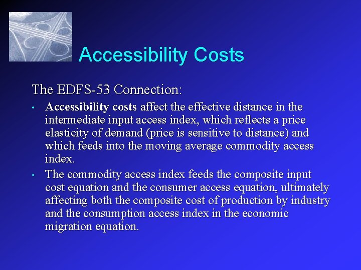
Accessibility Costs The EDFS-53 Connection: • • Accessibility costs affect the effective distance in the intermediate input access index, which reflects a price elasticity of demand (price is sensitive to distance) and which feeds into the moving average commodity access index. The commodity access index feeds the composite input cost equation and the consumer access equation, ultimately affecting both the composite cost of production by industry and the consumption access index in the economic migration equation.

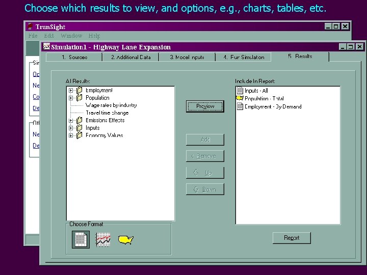
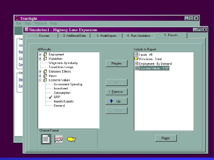
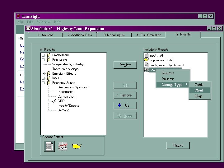
Choose which results to view, and options, e. g. , charts, tables, etc.

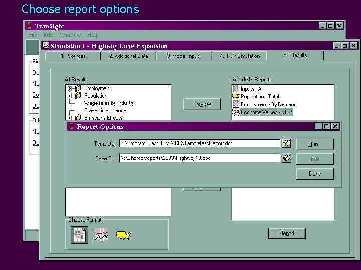
Choose report options

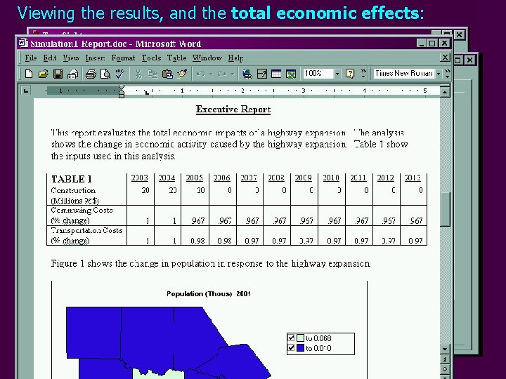
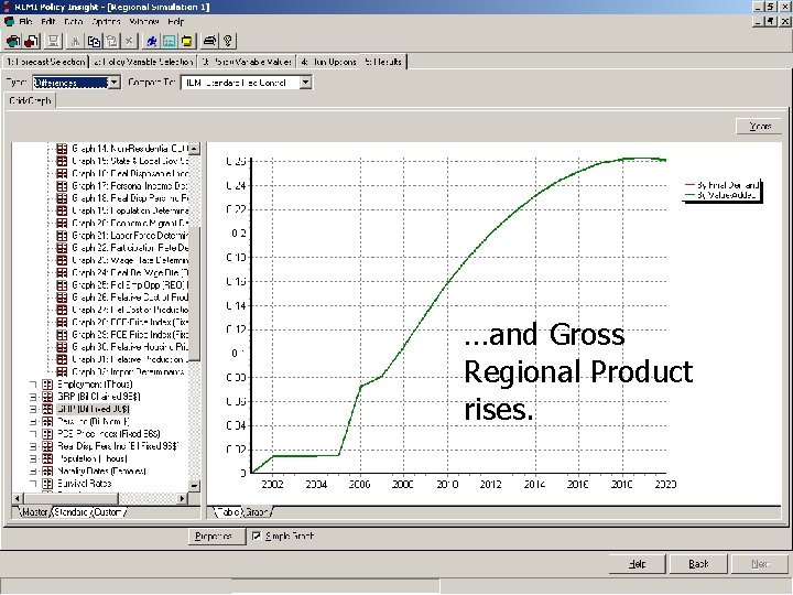
Viewing the results, and the total economic effects:

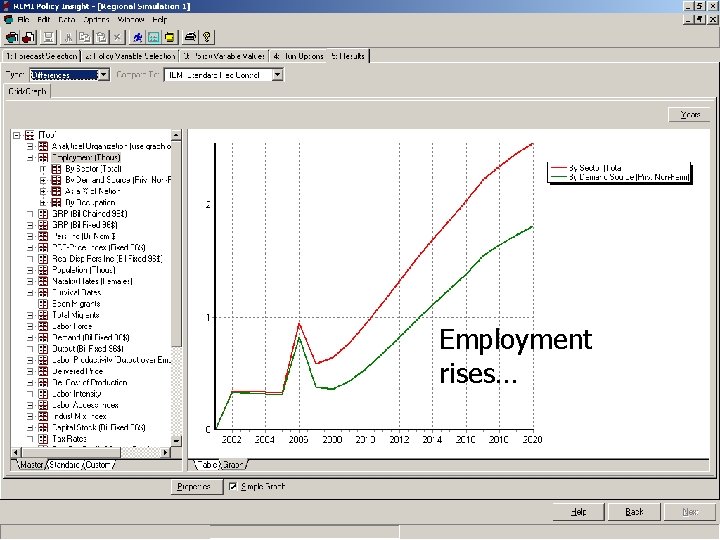
Employment rises… Total and private nonagricultural employment rises…

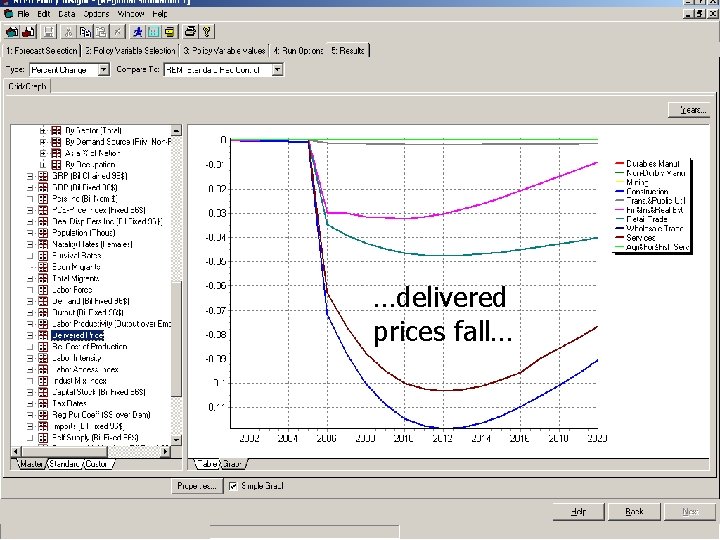
…delivered prices fall…

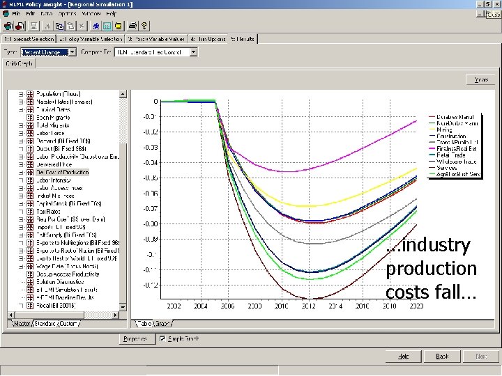
…industry production costs fall…

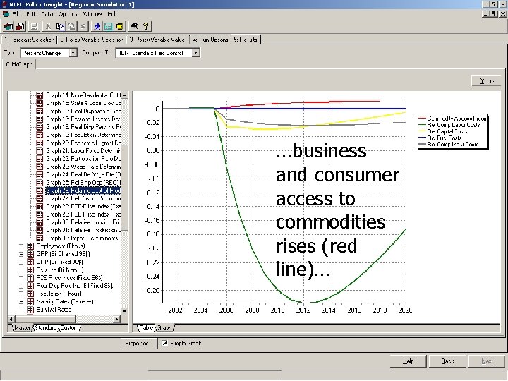
…business and consumer access to commodities rises (red line)…

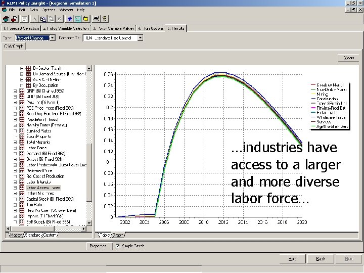
…industries have access to a larger and more diverse labor force…

…and Gross Regional Product rises.

Why REMI Tran. Sight? n Integrating transportation with economic and fiscal simulation models requires a sound theoretical basis. n REMI models are structurally complete, and built upon widely accepted economic theory published in rigorously refereed academic journal articles. n Yet the economic theory behind REMI Tran. Sight is accessible to any thoughtfu person.

Why REMI Tran. Sight? REMI has been involved in transportation planning for years. Below, a few examples (papers available upon request): n An Evolutionary New Economic Geography Model”; Wei Fan, Department of Economics, University of Michigan, Ann Arbor; Frederick Treyz and George Treyz, Regional Economic Models, Inc; Journal of Regional Science, Vol 40, No. 4, 2000 pp. 671 -695. n “Monopolistic Competition Estimates of Interregional Trade Flows in Services”, Frederick Treyz and Jim Bumgardner; Regional Cohesion and Competition in the Age of Globalization, June 2000. n “Productivity and Accessibility: Bridging Project-Specific and Macroeconomic Analyses of Transportation Investments”, Glen Weisbrod and Frederick Treyz; Journal of Transportation And Statistics, Vol. 1, No. 3, October 1998. n “NCHRP Report 463: Economic Implications of Congestion”; Glen Weisbrod, Donald Vary, George Treyz; Transportation Research Board – National Research Council; 2001.