ReliabilityBased List Decoding of Linear Block Codes Marc

Reliability-Based List Decoding of Linear Block Codes Marc Fossorier Department of Electrical Engineering University of Hawaii at Manoa, USA University of Waterloo, Canada April 26, 2004

Communication Channel: l l (N, K, dmin) binary linear block code. AWGN channel.

Maximum Likelihood Decoding: Find the codeword c which minimizes the discrepency metric: l l “Brute-force” decoding: Out of 2 K possible solutions, find the most probable (i. e. the codeword with minimum discrepency metric).

Suboptimum reliability-based decoding: l l Reorder the received values in decreasing reliability values: Use reliability information to reduce the search space (list decoding).

Two main families of reliability based decoding algorithms: Least reliable-based decoding: a lot of errors are likely to be confined in the least reliable positions => systematic covering of these positions. l Most reliable-based decoding: few errors are likely to be located in the most reliable positions => consider only error patterns of small Hamming weight in these positions. l

Least reliability-based decoding: l l Add predetermined error patterns with support in the least reliable positions to the hard decision of the received vector. Use an algebraic decoder to decode each constructed N-tuple. Select the most likely codeword among those generated by the decoder. Ex: GMD, Chase-type, …

Most reliability-based decoding: l l Determine or a few information sets from most reliable positions. Add predetermined error patterns of small Hamming weight to hard decision of the received vector in the information set. Re-encode each modified information set. Select the most likely codeword among those generated by the encoder.

A simple example for (6, 3, 3) code [1]: 1 0 0 0 1 1 c = (0, 0, 0, 0); G = 0 1 0 1 0 0 1 1 1 0 y = (2. 2, 0. 9, -0. 7, 0. 4, 0. 3, 0. 8); z = (2. 2, 0. 9, 0. 8, -0. 7, 0. 4, 0. 3) = p 1(y); 1 0 0 1 p 1(G) = 0 1 1 0 0 0 0 1 1 1 z. HD = (0, 0, 0, 1, 0, 0);

A simple example for (6, 3, 3) code [2]: 1 0 0 1 p 2(p 1(G)) = 0 1 1 0 0 0 1 1 r = p 2(z) = p 2(p 1(y)) ; In general, p 2(p 1(G)) is not in systematic form Þ Perform Gaussian elimination to obtain systematic form. b 0 = (0, 0, 1) => c 0 = b 0 p 2(p 1(G)) = (0, 0, 1, 1);

A simple example for (6, 3, 3) code [3]: Another technique to avoid p 2() is incomplete information set decoding: => 2 d decodings corresponding to d dependency occurrences. p 1(G) = 1 0 0 1 1 0 0 0 0 1 1 1 => b 0 = (0, 0, ? );

Reprocessing in most reliable basis: l The K most reliable independent positions define the most reliable basis (MRB). l Different strategies to reprocess low weight error patterns in MRB and create the list of codeword candidates. Two objectives: (1) Reach the MLD solution as early as possible. l (2) Recognize that the MLD solution has been tested.

Decoding costs: l l l List size M corresponding to the maximum number of tested error patterns (also useful to evaluate error performance). Genius G corresponding to the average number of tested error patterns before the MLD solution is found. Sufficiency number S corresponding to the average number of tested error patterns before the genius is recognized to have been reached. G < S < M

Conditions for optimality: l Useful to lower average decoding complexity (reduce S). Two types: (1) necessary conditions (NC) to know that a candidate or a subset of candidates are not optimal (save their decoding cost). (2) sufficient conditions (SC) to know that a candidate is optimal (save the decoding cost of the rest of the list). l

Resource: l A trivial lower bound on l r. HD = c = D 1 is 0. D 1 For c 1 to be a valid candidate, it shoud differ dmin - |D 1| from c in at least dmin positions. . v =

l Resource based on 1 codeword [Taipale-Pursley: IT 91]: s(v) r s(c) l Resource based on several codewords [Kasami: AAECC 99]: s(c 1) r s(c) s(v)

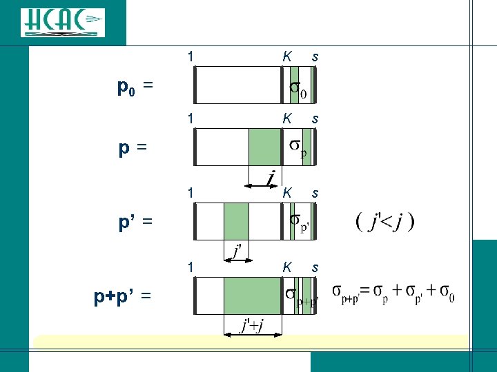
Strategies for error pattern reprocessing: 1 K b 0 = 1 K N 1 i K N => c 0 = 1 i K ei = b 0+ei = => ci =

Strategy-1 [Dorsch: IT 74]: l Reprocess c 0 in increasing a-priori discrepency value with respect to the MRB. e 1 = (0 0 … 0 0 1) => L 1 = | r. K | e 2 = (0 0 … 0 1 0) => L 2 = | r. K-1 | e 3 = (0 0 … 1 0 0) => L 3 = | r. K-2 | or (0 0 … 0 1 1) => L 3 = | r. K-1 | + | r. K | ? (originally designed for quantized values )

Improvement-1 [Battail-Fang: AT 86]: Update K disjoint ordered lists L(i) corresponding to error patterns with support in positions 1, …, i and with 1 in position-i (K-tuples). Example: r = (2. 2, 0. 9, -0. 7, 0. 8, 0. 4, 0. 3) Initialization: L(1): (<1>; 2. 2) L(2): (<2>; 0. 9) (all weight-1 patterns) L(3): (<3>; 0. 7) Candidate-1: (<3>; 0. 7)

List update: append to the last selected pattern in L(j) each suffix i of descendant lists L(i), i>j. L(1): (<1>; 2. 2); L(2): (<2>; 0. 9); L(3): Candidate-2: (<2>; 0. 9) List update: L(1): (<1>; 2. 2); L(2): L(3): (<23>; 1. 6);

Candidate-3: (<23>; 1. 6) List update: L(1): (<1>; 2. 2); L(2): L(3): Candidate-4: (<1>; 2. 2) List update: L(2): (<12>; 3. 1) L(3): (<13>; 2. 9) Problem: “ 1 out; K-i in” => memory overflow before MLD solution is reached. l

Improvement-2 [Valembois-Fossorier: CL 01]: Modifications: (1) Store ordered list A of processed patterns. (2) In each list L(i), store for pattern <i 1, …, im, i> the position p of pattern <i 1, …, im> in list A. “ 1 out; 1 in”: When [<i 1, …, im, i>; p] in L(i) is chosen as best candidate, find the pattern <j 1, …, jn> at position q>p in A with jn<i. Add [< j 1, …, jn, i>; q] in L(i) and <i 1, …, im, i> in A.

Strategy-2 [Han-Hartmann-Chen: IT 93]: Order the error patterns e not only with respect to their discrepency values over the MRB, but also by adding to them: There is no advantage in keeping K ordered lists Þ Regroup them into a single ordered list. Use SC, as well as NC based on R(w. H(e)).

l Although presented differently (binary tree), the algorithm proposed by Han-Hartmann-Chen is equivalent to Battail-Fang’s algorithm with the improved cost function. l The improvement proposed by Valembois-Fossorier can also be applied to this algorithm. Remaining problems: (1) Order in which patterns are reprocessed depends on each received sequence. (2) No performance analysis for fixed size list. .

Strategy-3 [Fossorier-Lin: IT 95]: l Process the error patterns into families F(w) of increasing Hamming weight w. l For the family of Hamming weight w, use: The SC and NC benefit from the structure: Example: SC after completing F(2) l

l l OSD-i: reprocessing of families F(0), F(1), …, F(i). Phase-j of OSD-i: reprocessing of family F(j). Number of candidate codewords in phase-j: Maximum list size of OSD-i:

Reprocessing within each family: [Fossorier-Lin: IT 95]: 0000… 000111 0000… 001011 0000… 010011 0000… 100011 … l [Gazelle-Snyders: IT 97]: 0000… 000111 0000… 001011 0000… 001101 0000… 001110 … Slightly more efficient for some list sizes. l

l Structure also useful to evaluate error performance for finite list sizes (OSD-i): with: PA: Probability algorithm is in error. PMLD: Probability MLD is in error (tight bounds exists) Plist: Probability that MLD solution is not in the list processed by the algorithm. l Interesting case: Plist << PMLD

Evaluation of Plist based on order statistics [Agrawal-Vardy: IT 00; Fossorier-Lin: IT 01] Assume j hard decision errors out of N received values ordered in decreasing reliability values: l l l Remaining N-j correct hard decisions ordered in decreasing reliability values: Order statistics of ‘s and ‘s known.

l Density function of

l Density function of

l Double integration to compute:

l Assume OSD-i: Plist = Pr [at least (i+1) errors in the MRB] l Assuming no dependency occurrences and j hard decision errors: l If d dependency occurrences: These probabilities can be evaluated numerically with double integrals.

with: PD(d): Probability K-th most reliable independent position is found at the ordered position-K+p. This probability can be easily evaluated numerically, or expressed from [Fossorier-Lin: IT 95].

(128, 64, 22) e. BCH code: i=0: |L| = 1 i=1: |L| = 65 i=2: |L| = 2, 081 i=3: |L| = 43, 745 i=4: |L| = 679, 121 ~ 219. 4

(128, 64, 22) e. BCH code:

Iterative information set decoding (IISD) [Fossorier-IT 02]: l l l Provide a level of flexibility between OSD-i and OSD(i+1) with systematic reprocessing strategy and tight error performance analysis. Assume that if at least (i+1) errors in MRB, then it is likely that most reliable positions outside MRB can be error free. Assign highest reliability values to them and build the corresponding MRB.

1 K p N r. HD = OSD-i fails 1 p-K r. HD(2) = K p N OSD-i succeeds Repeat iteratively the processus. If no dependency occurrences, the processus terminates after exactly iterations and 1 termination phase. At most 2 MRBs of size K need to be constructed.

l If no dependency occurrences, the list size before the termination step is exactly for IISD-i: (at iteration-l, OSD-i for MRB of size K-(l-1)(p-K)). Dependency occurrences make the number of iterations (and hence the list size) dependent on the received sequence. However, it can be proved that a negligible degradation in error performance is induced by performing only iterations. l

l Performance analysis of IISD-(i, p): Plist = Pr [at least (i+1) errors in the MRB and at least (i+2) errors in p MRPs] (with respect to initial ordering). This expression can be computed based on four-fold integrals corresponding to, for j transmission errors: Dependency occurrences can be ignored in evaluating Plist as it is probable enough that the p MRPs contain an information set (roughly 1 -2 -(p-K)).

Box-and-match algorithm (BMA) [Valembois-Fossorier: ITsub, ISIT 02]: Observe that all previous algorithms have zero memory cost: => Try to store and use information obtained during OSD-i to cover additional error patterns. l Use matching techniques already applied in cryptanalysis [Stern: LNCS 89; Canteaut-Chabaud: IT 98]. l Related approach proposed in [Dumer: IT 99, IT 01]. Compared to that approach, BMA generally has lower computation complexity, but higher memory requirement. l

l Phase-j of BMA-(i, s) : Correct all error patterns with either j errors over the MRB, or 2 j-1 or 2 j errors over the s MRPs. 1 K s N r. HD = Note that several patterns with j errors over the MRB can be corrected at a phase j’ < j (important fact for NC and SC). l

l For p+p’ to have weight 2 j-1 or 2 j, For must have weight j – j ’-1 or j - j’. l The error patterns in each phase of BMA-(i, s) are processed in a very structured manner so that the previous description allows to cover all error patterns of weight 2 j-1 and 2 j over the s MRPs. More precisely, if all the non zero positions over the MRB in a pattern (s-tuple) p are less reliable than those in a pattern p’, then p is processed before p’.

l Phase-j of BMA-(i, s): (1) Reprocessing: Process all patterns (s-tuples) p of Hamming weight j over the MRB (same as phase-j of OSD-i), and store p in the box B[ ]. (2) Matching: For all patterns p’ of Hamming weight j’<j over the MRB, for all (s-K)-tuples of Hamming weight j-j’-1 or j-j’ and all patterns p’’ retrieved from the box B[ ], process p’’+ p’.

l List size for BMA-(i, s): Reprocessing: Matching (on average): l l Memory requirement for BMA-(i, s): SC and NC of phase-j of BMA-i very powerful compared to that of phase-j of OSD-i (roughly of the strength of phase-(2 j-1) of OSD-i)

l Performance analysis of BMA-(i, s): Plist = Pr [at least (i+1) errors in the MRB and at least (2 i+1) errors in s MRPs] This expression can be computed based on four-fold integrals corresponding to, for j transmission errors: Dependency occurrences can be ignored in evaluating Plist as it is probable enough that the s MRPs contain an information set (roughly 1 -2 -(s-K)).

e. BCH (128, 64, 22):

BZ (192, 96, 28):

e. BCH (256, 187, 20):

e. BCH (512, 475, 10):

BMA with IISD [Fossorier-Valembois: ITW 02]: l Combine BMA-(i; s) and IISD-(i; p) into IBMA(i; s; p): 1 K r. HD = N 0 1 r. HD(2) = s p K 0 s p N …

l Performance analysis of IBMA-(i, s, p): Plist = Pr [at least (i+1) errors in the MRB and at least (2 i+1) errors in s MRPs and at least (2 i+2) errors in p MRPs] This expression can be computed based on six-fold integrals corresponding to, for j transmission errors:

Six-fold integrals are computationally expensive to evaluate. Instead, we can use: Plist Pr [at least (i+1) errors in the MRB and at least (2 i+2) errors in p MRPs]. This upper bound remains tight for small values of p-s and can be evaluated based on four-fold integrals corresponding to, for j transmission errors:

BZ (192, 96, 28):

BZ (192, 96, 28):

Conclusions for Binary Codes: l IBMA-(i; s; p) allows to achieve practically optimum decoding of a (192, 96, 28) binary linear block code. l The next meaningful benchmark for a soft decision decoding algorithm is practically optimum decoding of the (256, 131, 38) e. BCH code (with performance analysis available).

Application to Non Binary Codes: l Use binary image of non-binary code and apply previous approach: an (N, K) code over GF(2 m) has an (Nm, Km) code as binary image). l Ordering could be applied at the symbol level but despite structural advantages, such approaches have reveal less computationally efficient.

RS (255, 239, 17):

RS (255, 239, 17):

RS (255, 239, 17): Algorithm log 2(list size) log 2(# CB- patterns) log 2(memory) SER OSD(1) 10. 9 0 7. 88 OSD(2) 20. 8 0 11. 73 BMA(1, 22) 10. 9 11. 9 22. 0 11. 72 BMA(2, 22) 20. 9 21. 8 22. 0 19. 24 ITBMA(1, 22, 10) 12. 9 – 18. 5 13. 9 – 19. 5 22. 0 15. 51 ITBMA(2, 22, 10) 22. 9 – 28. 5 23. 8 – 29. 4 22. 0 22. 90 Algebraic decoding: SER = 9; MLD: SER > 17.