Reliability Engineering RELIABILITY 1 Definition of Reliability The

可靠度 程 Reliability Engineering RELIABILITY 1

Definition of Reliability The probability, at a desired confidence level, that a device will perform a specified function, without failure, under stated conditions, for a specified period of time RELIABILITY 2
 Ø“The probability of a product performing without failure a specified function")
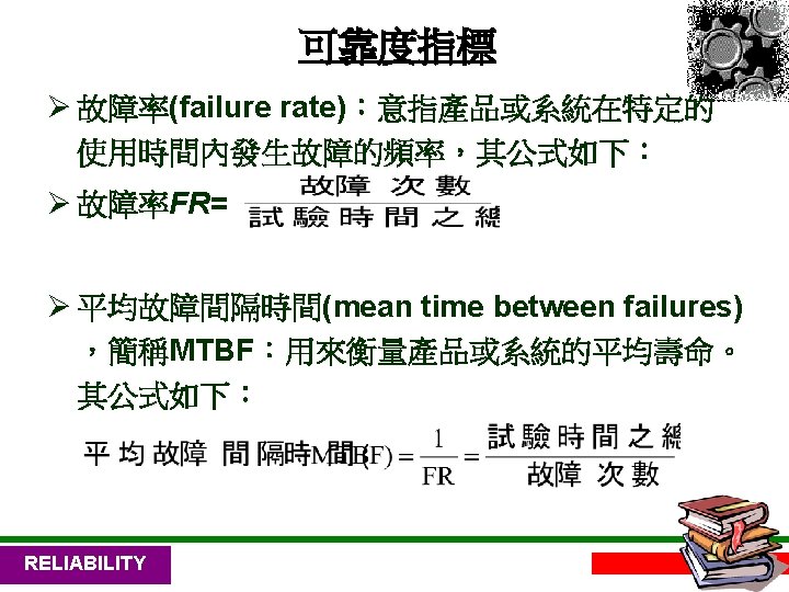
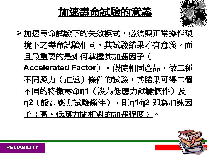
可靠度 程定義 ØDefinition(定義) Ø“The probability of a product performing without failure a specified function under given conditions for a specified period of time”(所謂可靠度是指特定產品在給定之操作 環境及條件下,能成功的發揮其應有功能至一 給定時間之機率) Ø設給定的時間為T,以數學式表示可靠度之形 式為: RELIABILITY 3

可靠度 程定義 ØIn two formats ØProbability that system will perform on a given trial Ø 99. 999% for telephone system (Five-9 system) ØFrequency of successful performances of a system in a given number of attempts. Ø 10, 000 operating hours RELIABILITY 4
 ØProbability Øfrequency of successful uses out of a certain number")
可靠度 程定義 ØThree dimensions(三種尺度) ØProbability Øfrequency of successful uses out of a certain number of attempts ØLikelihood of an item lasting a given amount of time ØFailure ØA situation in which an item does not perform as intended ØOperating conditions ØHow the product should be used? ØWhat is “normal operating conditions” RELIABILITY 5

Reliability Basics Reliability cannot be tested into a product It must be designed and manufactured into it Testing only indicates how much reliability is in the product 可靠度無法藉由檢驗進入產品 它必須被設計和製造進去 試驗僅能指出產品裡俱有多少的可靠度 RELIABILITY 6

Customer’s Definition of Reliability A reliable product: 可靠的產品 One that does what the customer wants, when the customer wants to do it 可靠的產品是顧客想要的時候, 它都能達成客戶想要的 RELIABILITY 7
 Ømeets the specification when new Ø Reliability Øcontinues to")
Quality vs Reliability Ø Quality(品質) Ømeets the specification when new Ø Reliability Øcontinues to meet the specification through a period of use Ø “customer expectations” vs “specification” RELIABILITY 8
 current performance Reliability future performance Test time t=0")
Quality vs Reliability Criteri Quality Objective(目的) current performance Reliability future performance Test time t=0 [ 0, t ) Decision defect failure defective rate (%) failure rate(%/ yr) Relevant process manufacturing, inspection system design, materials, component Tool for SPC, TQC FMEA, FTA improvement 6 Sigma failure analysis, design review Test method Inspection life testing until failure Pass of no pass performance measure (MTTF, failure rate ) Classification Test result RELIABILITY 9

Probability of Occurrence Infant Mortality New units load After Infant Mortality strength Failure region load strength Failure region Applied or Failure Stress RELIABILITY 13

Wear Out After wear-out New units load strength Failure region RELIABILITY load strength Failure region 14

可靠性試驗 RELIABILITY 17
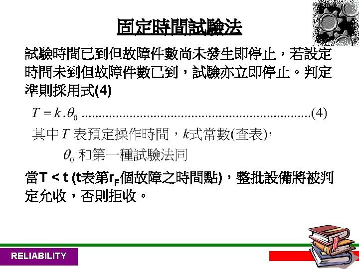
 ˙固定個數試驗法(定數截尾試驗) (Fixed Failure Numbers Testing) ˙固定時間試驗法(定時截尾試驗) (Fixed Time Testing)")
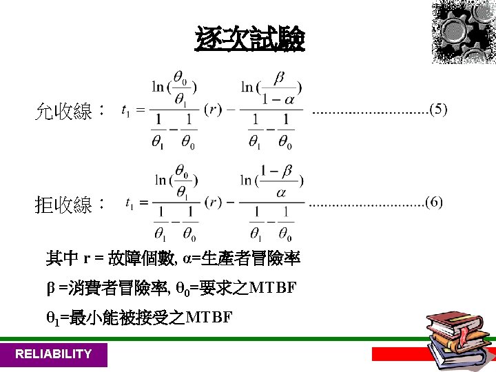
可靠性試驗方法 Ø 固定長度試驗法(Fixed Length Testing) ˙固定個數試驗法(定數截尾試驗) (Fixed Failure Numbers Testing) ˙固定時間試驗法(定時截尾試驗) (Fixed Time Testing) Ø 逐次試驗法 (Sequential Testing) Ø 加速壽命試驗法(Accelerated Life Testing) RELIABILITY 24

加速壽命試驗 References: Kececioglu, D. and Jacks, J. Q. , “The Arrhenius, Eyring, inverse power law and Combination models in accelerated testing”, Reliability Engineering, (1983) Parker, T. P. and Webb, C. W. , “A Study of Failure Identified During Board Level Environmental Stress Testing, ” IEEE Transaction on Components, Hybrids and Manufacturing Technology, Vol. 15, No. 6, pp. 1086 -1092(1992). RELIABILITY 43

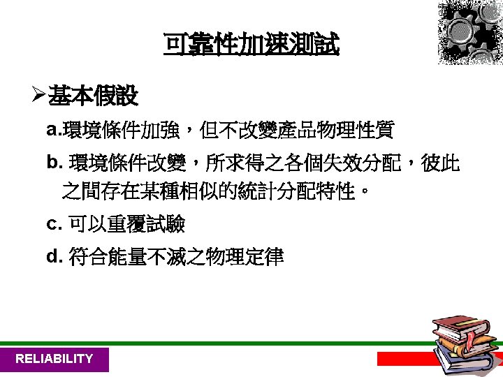
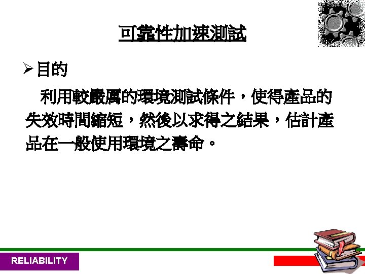
可靠性加速測試方法 Ø 目的 Ø 基本假設 Ø 加速試驗模式 Ø Inverse Power Model Ø Arrhenius Model for Thermal Aging Ø 時間轉換法 Ø 貝氏法則 RELIABILITY 44
物理模式 * Inverse Power Law * Arrhenius Law (二)統計模式 * Time Transformation Models")
加速試驗模式 (一)物理模式 * Inverse Power Law * Arrhenius Law (二)統計模式 * Time Transformation Models * Baye’s Method RELIABILITY 50
")
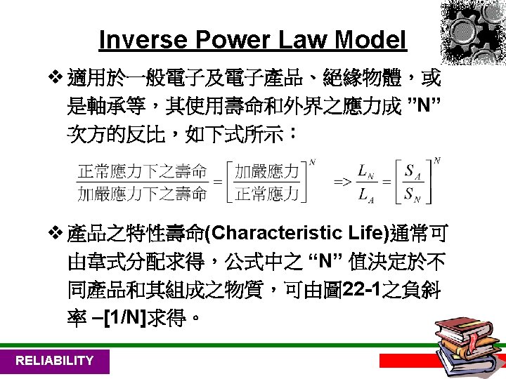
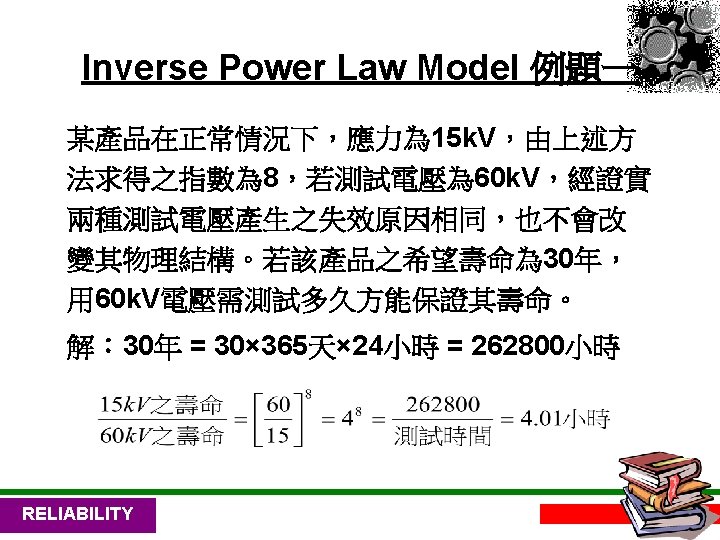
Inverse Power Law Model Inverse Power Law Relationship Introduction The inverse power law (IPL) model (or relationship) is commonly used for non-thermal accelerated stresses and is given by: (1) where: L represents a quantifiable life measure, such as mean life, characteristic life, median life. V represents the stress level. K is one of the model parameters to be determined, (K > 0). n is another model parameter to be determined. RELIABILITY 54

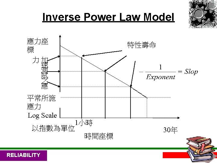
Inverse Power Law Model The inverse power law appears as a straight line when plotted on a log-log paper. The equation of the line is given by: (2) Plotting methods are widely used in estimating the parameters of the inverse power law relationship since obtaining K and n is as simple as finding the slope and the intercept on Eqn. (2). . Graphical look at the IPL relationship (log-log scale) RELIABILITY 55

Inverse Power Law Model A Look at the Parameter n The parameter n in the inverse power relationship is a measure of the effect of the stress on the life. As the absolute value of n increases, the greater the effect of the stress. Negative values of n indicate an increasing life with increasing stress. An absolute value of n approaching zero indicates small effect of the stress on the life, with no effect (constant life with stress) when n = 0. Life vs. stress for different values of n. RELIABILITY 56

Inverse Power Law Model For the IPL relationship the acceleration factor is given by: where: LUSE is the life at use stress level. LAccelerated is the life at the accelerated stress level. Vu is the use stress level. VA is the accelerated stress level. . RELIABILITY 57

Inverse Power Law Model Example 1 The inverse power law model was found to apply to a crush test performed on an implantable electrode. It was estimated that the electrode could be subjected to crush forces of approximately 4 lbf when implanted in the human body (normal use conditions). When subjected to accelerated crush test in the laboratory, the total cycles to failure were 35, 000 cycles. The accelerated crush force was 8 lbf. The results of accelerated tests performed in the test lab indicate that an (N) factor of 8 applies. Determine the expected cycles to failure under normal use conditions. How would you determine the (N) factor of 8? RELIABILITY 58

Inverse Power Law Model Solution: Assuming the shape parameters of the probability distribution at normal use conditions and at accelerated stress conditions are the same, the inverse power relationship can be written as: The (N) factor is determined empirically by conducting two tests at different stress levels. Let us assume that applied Stress 1 = 8 lbf and Stress 2 = 10 lbf. At eight-lbf stress we obtain 35, 000 cycles to failure and at ten-lbf stress we get 5872 cycles to failure. Number of cycles Test 1 = B(Stress 1)-N Number of cycles Test 2 = B(Stress 2)-N Taking the Log on both sides of the equation we get: RELIABILITY 59
")
Arrhenius Model for Thermal Aging Arrhenius Relationship Introduction The Arrhenius life-stress model (or relationship) is probably the most common life-stress relationship utilized in accelerated life testing. It has been widely used when the stimulus or acceleration variable (or stress) is thermal (i. e. temperature). It is derived from the Arrhenius reaction rate equation proposed by the Swedish physical chemist Svandte Arrhenius in 1887. The Arrhenius reaction rate equation is given by: where: • R is the speed of reaction. • A is an unknown nonthermal constant. • EA is the activation energy (e. V). • K is the Boltzman’s constant (8. 617385 x 10 -5 e. V K-1). • T is the absolute temperature (Kelvin). RELIABILITY 60

Arrhenius Model for Thermal Aging The activation energy is the energy that a molecule must have to participate in the reaction. In other words, the activation energy is a measure of the effect that temperature has on the reaction. The Arrhenius life-stress model is formulated by assuming that life is proportional to the inverse reaction rate of the process, thus the Arrhenius lifestress relationship is given by: (1) where: • L represents a quantifiable life measure, such as mean life, characteristic life, median life. • V represents the stress level (formulated for temperature and temperature values in absolute units i. e. degrees Kelvin or degrees Rankine). • C is one of the model parameters to be determined, (C > 0). • B is another model parameter to be determined. RELIABILITY 61

Arrhenius Model for Thermal Aging The Arrhenius relationship can be linearized and plotted on a life vs. stress plot, also called the Arrhenius plot. The relationship is linearized by taking the natural logarithm of both sides in Eqn. (1) or: (1) Depending on the application (and where the stress is exclusively thermal), the parameter B can be replaced by: Note that in this formulation, the activation energy must be known a priori. If the activation energy is known there is only one model parameter remaining, C. Because in most real life situations this is rarely the case, all subsequent formulations will assume that this activation energy is unknown and treat B as one of the model parameters. As it can be seen in Eqn. (1 ), B has the same properties as the activation energy. In other words, B is a measure of the effect that the stress (i. e. temperature) has on the life. The larger the value of B, the higher the dependency of the life on the specific stress. Parameter B may also take negative values. In that case, life is increasing with increasing stress. An example of this would be plasma filled bulbs, where low temperature is a higher stress on the bulbs than high temperature. RELIABILITY 62

Arrhenius Model for Thermal Aging Behavior of the parameter B. RELIABILITY 63

Arrhenius Model for Thermal Aging Arrhenius Acceleration Factor Most practitioners use the term acceleration factor to refer to the ratio of the life (or acceleration characteristic) between the use level and a higher test stress level or: For the Arrhenius model this factor is: Thus, if B is assumed to be known a priori (using an activation energy), the assumed activation energy alone dictates this acceleration factor! RELIABILITY 64

時間轉換法 Time-Varying Stresses: The Cumulative Damage Model Traditionally, accelerated tests that use a time-varying stress application have been used to assure failures quickly. This is highly desirable given the pressure on industry today to shorten new product introduction time. The most basic type of time-varying stress test is a step-stress test. In step-stress accelerated testing, the test units are subjected to successively higher stress levels in predetermined stages and thus follow a time-varying stress profile. The units usually start at a lower stress level and at a predetermined time, or failure number, the stress is increased and the test continues. The test is terminated when all units have failed, when a certain number of failures are observed or when a certain time has elapsed. Step-stress testing can substantially shorten the reliability test's duration. In addition to step-stress testing, there are many other types of time-varying stress profiles that can be used in accelerated life testing. However, it should be noted that there is more uncertainty in the results from such time -varying stress tests than from traditional constant stress tests of the same length and sample size. When dealing with data from accelerated tests with time-varying stresses, the lifestress relationship must take into account the cumulative effect of the applied stresses. Such a model is commonly referred to as a “cumulative damage” or “cumulative exposure” model. Nelson [31 ] defines and presents the derivation and assumptions of such a model. RELIABILITY 66

時間轉換法 Time-Varying Stress Model Formulation To formulate the cumulative exposure/damage model, consider a simple step-stress experiment where an electronic component was subjected to a voltage stress, starting at 2 V (use stress level) and increased to 7 V in stepwise increments as shown in Figure 1. The following steps, in hours, were used to apply stress to the products under test: 0 to 250, 2 V; 250 to 350, 3 V; 350 to 370, 4 V; 370 to 380, 5 V; 380 to 390, 6 V; and 390 to 400, 7 V. RELIABILITY 67

時間轉換法 In this example, eleven units were available for the test. All eleven units were tested using this same stress profile. Units that failed were removed from the test and their total times on test were recorded. The following times-tofailure were observed in the test, in hours: 280, 310, 330, 352, 360, 366, 371, 374, 378, 381 and 385. The first failure in this test occurred at 280 hours when the stress was 3 V. During the test, this unit experienced a period of time at 2 V before failing at 3 V. If the stress were 2 V, one would expect the unit to fail at a time later than 280 hours, while if the unit were always at 3 V, one would expect that failure time to be sooner than 280 hours. The problem faced by the analyst in this case is to determine some equivalency between the stresses. In other words, what is the equivalent of 280 hours (with 250 hours spent at 2 V and 30 hours spent at 3 V) at a constant 2 V stress or at a constant 3 V stress? RELIABILITY 68

時間轉換法 範例 Voltage Stress Example An electronic component was subjected to a voltage stress, starting at 2 V (use stress level) and increased to 7 V in stepwise increments. The following steps, in hours, were used to apply stress to the products under test: 0 to 250, 2 V; 250 to 350, 3 V; 350 to 370, 4 V; 370 to 380, 5 V; 380 to 390, 6 V; and 390 to 400, 7 V. This profile is represented graphically next. The objective of this test was to determine the B(10) life of these components at the normal use stress level of 2 V. RELIABILITY 69

時間轉換法 範例 In this experiment, the overall test time was 385 hrs. If the test had been performed at use conditions, one would expect the test duration to be approximately 1700 hrs if the test were run until all units failed Eleven units were available for the test. All eleven units were tested using the same stress profile. Units that failed were removed from the test and their total time on test recorded. The following times-to-failure were observed in the test, in hours: 280, 310, 330, 352, 360, 366, 371, 374, 378, 381 and 385. RELIABILITY 70

時間轉換法 範例 RELIABILITY 71

時間轉換法 範例 RELIABILITY 72
 life at the 2 V use stress level can be")
時間轉換法 範例 The B(10) life at the 2 V use stress level can be calculated with ALTA's Quick Calculation Pad (QCP), as shown next. RELIABILITY 73

Some practical guidelines for using ALT methods ‧Accelerated test programs should be planned and conducted by teams including individuals who are knowledgeable about the design and manufacturing of the product, its use environment, the physical/chemical/mechanical aspects of the failure mode(s), and the statistical aspects of the design and analysis of reliability experiments. ‧Accelerating variables should be chosen to correspond with variables that cause actual failures. Look for previous attempts to accelerate failure mechanisms similar to the ones of interest. There are many research reports and papers that have been published in the physics of failure literature. ‧Accelerated tests should be designed, as much as possible, to minimize the amount of extrapolation required. High levels of accelerating variables can cause extraneous failure modes that would never occur at use-levels of the accelerating variables. If extraneous failures are not recognized and properly handled, they can lead to incorrect conclusions. Also, be aware that acceleration relationships may not always be accurate enough over a wide range of stresses. RELIABILITY 82

Some practical guidelines for using ALT methods ‧The goal of an accelerated test should be used to obtain information about one particular, relatively simple failure mechanism. Multiple failure modes with different acceleration rates will invalidate the test model. It has been shown that simple acceleration models with the right shape are generally more useful than elaborate multi-parameter models. ‧In some test cases an accelerating variable like temperature may cause deceleration of another variable e. g. humidity. For this reason critical variables, which may be decelerated as a result of the test (and could cause failures in the field), should be controlled. ‧Ideally, samples used for accelerated testing come from actual production units manufactured by manufacturing operators, under actual production conditions, using qualified parts and raw materials. However, to be able to test as early as possible, we may want to use prototype units build by trained technicians in the lab. This trade-off between design speed and design cost (we may have to redo the test on final production units) is acceptable if the prototypes reflect, as much as possible, the variabilities that will be present in actual production e. g. variability in parts, raw materials, production processes, production equipment, production operators, etc. RELIABILITY 83
- Slides: 85