Reliability and Controls for Project X and Applications

Reliability and Controls for Project -X and Applications to Accelerator Driven Systems Sampriti Bhattacharyya, The Ohio State University Supervisors: RK Yedavalli (OSU), Aseet Mukherjee(FNAL), Jim Kerby (ANL)

Contents Reliability q q q Reliability & Its Importance Tools &software Failure Distributions Project X Reliability Methods of Modeling Data Validation against SNS Controls q Reliability and controls are particular importance to Accelerator Driven Syste

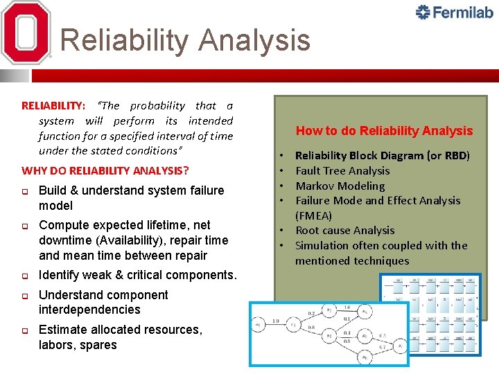
Reliability Analysis RELIABILITY: “The probability that a system will perform its intended function for a specified interval of time under the stated conditions” WHY DO RELIABILITY ANALYSIS? q q q Build & understand system failure model Compute expected lifetime, net downtime (Availability), repair time and mean time between repair Identify weak & critical components. Understand component interdependencies Estimate allocated resources, labors, spares How to do Reliability Analysis Reliability Block Diagram (or RBD) Fault Tree Analysis Markov Modeling Failure Mode and Effect Analysis (FMEA) • Root cause Analysis • Simulation often coupled with the mentioned techniques • •

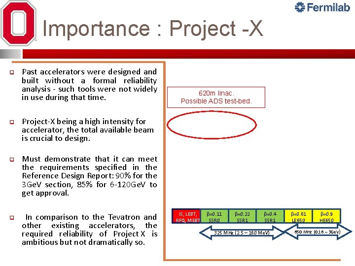
Importance : Project -X q q Past accelerators were designed and built without a formal reliability analysis - such tools were not widely in use during that time. 620 m linac. Possible ADS test-bed. Project-X being a high intensity for accelerator, the total available beam is crucial to design. Must demonstrate that it can meet the requirements specified in the Reference Design Report: 90% for the 3 Ge. V section, 85% for 6 -120 Ge. V to get approval. In comparison to the Tevatron and other existing accelerators, the required reliability of Project X is ambitious but not dramatically so. IS, LEBT, RFQ, MEBT b=0. 11 SSR 0 b=0. 22 SSR 1 b=0. 4 SSR 1 325 MHz (2. 5 – 160 Me. V) b=0. 61 LE 650 b=0. 9 HE 650 MHz (0. 16 – 3 Ge. V )

Accelerator Reliability Work Though no extensive systematic analysis has been much carried out on reliability of accelerators, there has been some work done in this field. A reliability study of the Spallation Neutron Source (SNS) has been done using a spreadsheet (Oak Ridge National Laboratory), and a customized reliability software called Avail. Sim was developed for the proposed International Linear Collider (SLAC). Out present work on reliability of Project-X uses a commercial simulation software called Availability Work. Bench (AWB) by Isograph. Data has been validation against SNS reliability results.

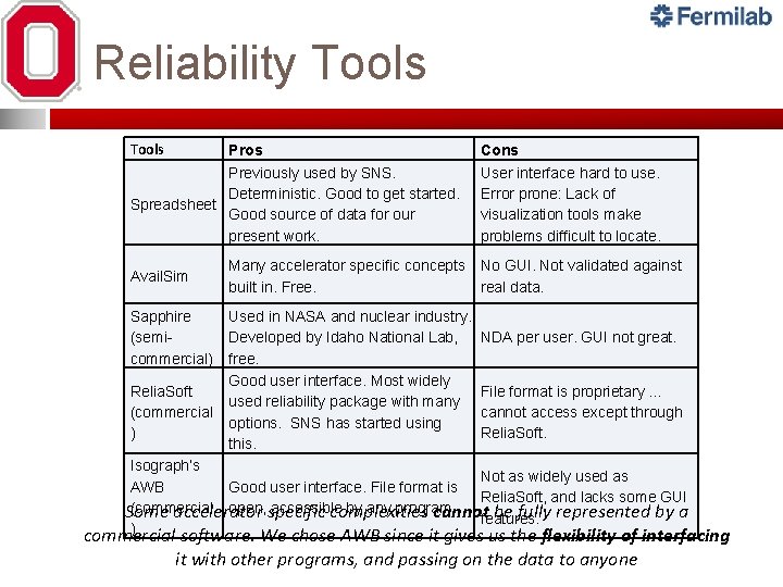
Reliability Tools Pros Previously used by SNS. Deterministic. Good to get started. Spreadsheet Good source of data for our present work. Avail. Sim Sapphire (semicommercial) Relia. Soft (commercial ) Cons User interface hard to use. Error prone: Lack of visualization tools make problems difficult to locate. Many accelerator specific concepts No GUI. Not validated against built in. Free. real data. Used in NASA and nuclear industry. Developed by Idaho National Lab, free. Good user interface. Most widely used reliability package with many options. SNS has started using this. NDA per user. GUI not great. File format is proprietary … cannot access except through Relia. Soft. Isograph’s Not as widely used as AWB Good user interface. File format is Relia. Soft, and lacks some GUI (commercial open, accessible by any program. Some accelerator specific complexities cannotfeatures. be fully represented by a ) commercial software. We chose AWB since it gives us the flexibility of interfacing it with other programs, and passing on the data to anyone

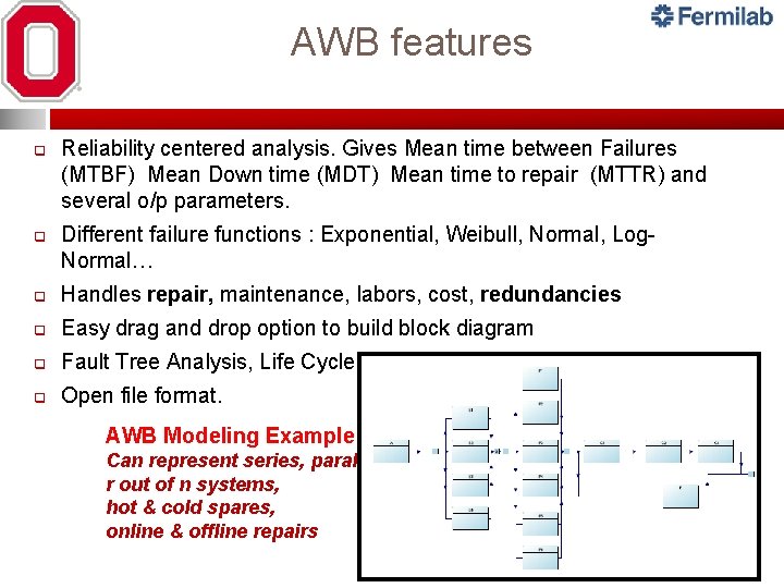
AWB features q q Reliability centered analysis. Gives Mean time between Failures (MTBF) Mean Down time (MDT) Mean time to repair (MTTR) and several o/p parameters. Different failure functions : Exponential, Weibull, Normal, Log. Normal… q Handles repair, maintenance, labors, cost, redundancies q Easy drag and drop option to build block diagram q Fault Tree Analysis, Life Cycle cost, Weibull Anaylsis. q Open file format. AWB Modeling Example Can represent series, parallel, r out of n systems, hot & cold spares, online & offline repairs

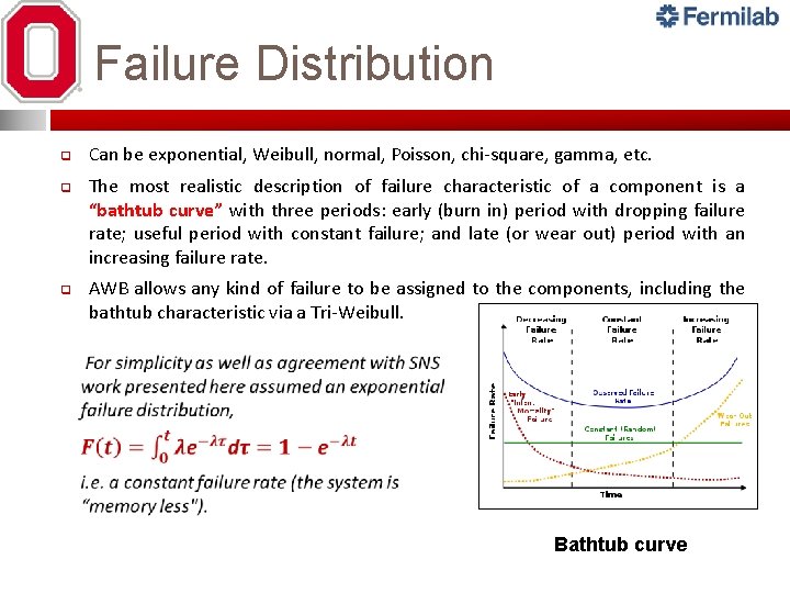
Failure Distribution q q q Can be exponential, Weibull, normal, Poisson, chi-square, gamma, etc. The most realistic description of failure characteristic of a component is a “bathtub curve” with three periods: early (burn in) period with dropping failure rate; useful period with constant failure; and late (or wear out) period with an increasing failure rate. AWB allows any kind of failure to be assigned to the components, including the bathtub characteristic via a Tri-Weibull. Bathtub curve

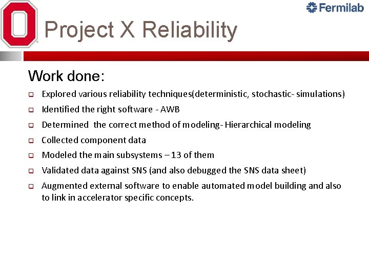
Project X Reliability Work done: q Explored various reliability techniques(deterministic, stochastic- simulations) q Identified the right software - AWB q Determined the correct method of modeling- Hierarchical modeling q Collected component data q Modeled the main subsystems – 13 of them q Validated data against SNS (and also debugged the SNS data sheet) q Augmented external software to enable automated model building and also to link in accelerator specific concepts.

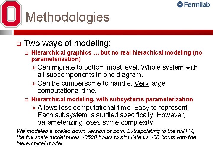
Methodologies q Two ways of modeling: q Hierarchical graphics … but no real hierachical modeling (no parameterization) Ø Can migrate to bottom most level. Whole system with all subcomponents in one diagram. Ø Can be cumbersome to handle. Very large computational time. q Hierarchical modeling, with subsystems parameterization Ø Allows less computational time. Easy to represent. Each subsystem is studied specifically. However, parameterizing loses some complexity. We modeled a scaled down version of both. Extrapolating to the full PX, the full scale model takes ~3500 hours to simulate vs ~30 hours with the hierarchical model.

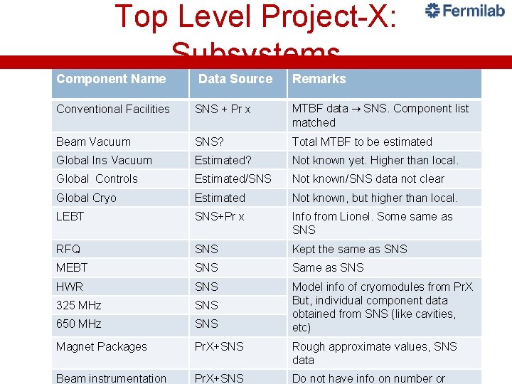
Top Level Project-X: Subsystems Component Name Data Source Remarks Conventional Facilities SNS + Pr x MTBF data → SNS. Component list matched Beam Vacuum SNS? Total MTBF to be estimated Global Ins Vacuum Estimated? Not known yet. Higher than local. Global Controls Estimated/SNS Not known/SNS data not clear Global Cryo Estimated Not known, but higher than local. LEBT SNS+Pr x Info from Lionel. Some same as SNS RFQ SNS Kept the same as SNS MEBT SNS Same as SNS HWR SNS 325 MHz SNS 650 MHz SNS Model info of cryomodules from Pr. X But, individual component data obtained from SNS (like cavities, etc) Magnet Packages Pr. X+SNS Rough approximate values, SNS data Beam instrumentation Pr. X+SNS Do not have info on number or

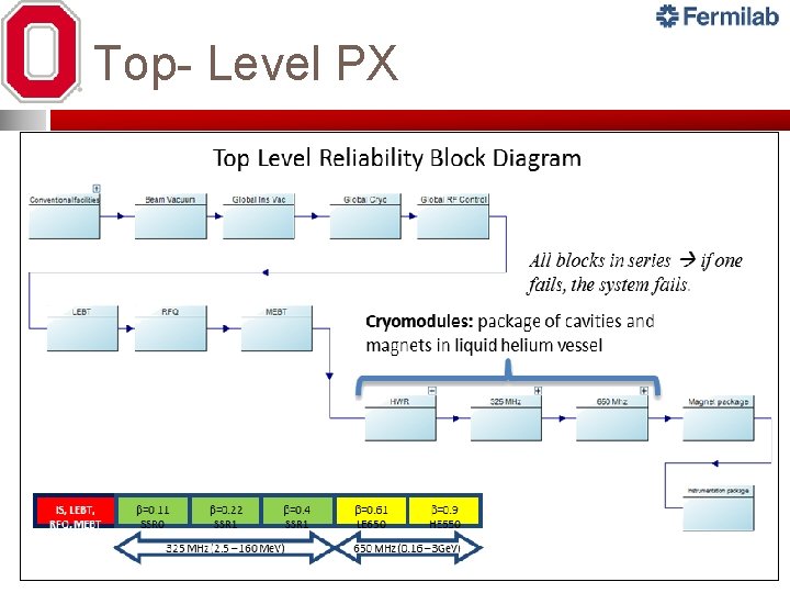
Top- Level PX

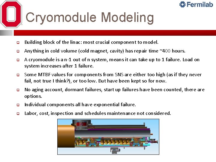
Cryomodule Modeling q Building block of the linac: most crucial component to model. q Anything in cold volume (cold magnet, cavity) has repair time ~400 hours. q q q A cryomodule is a n-1 out of n system, means it can take up to 1 failure. Load on system increases after 1 failure. Some MTBF values for components from SNS are either too high (as if they never fail, not true I think? ), or too low. But have been kept so for now. No aging account, dormant failures, start up failures have been counted, there are options. q Individual components all have exponential failure. q Labor, cost, inspection and schedules maintenance not considered.

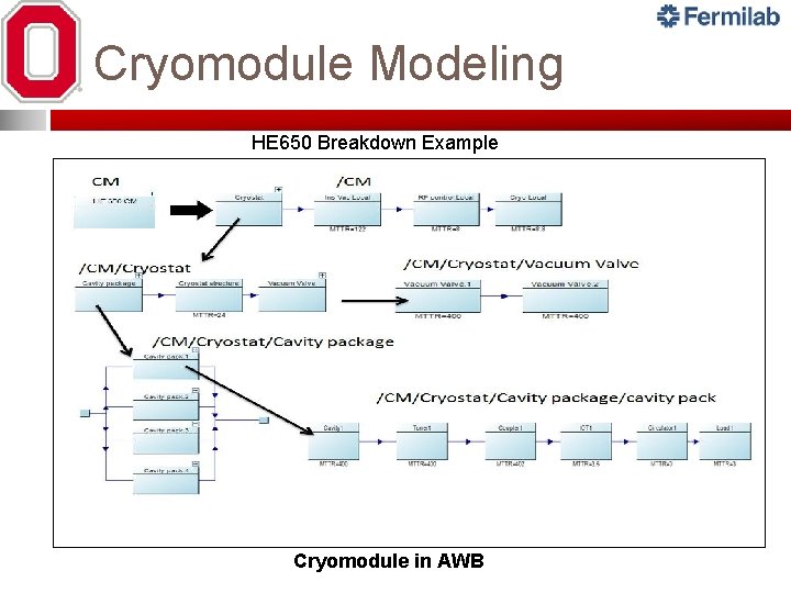
Cryomodule Modeling HE 650 Breakdown Example Cryomodule in AWB

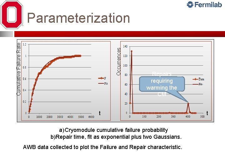
Occurrences Cumulative Failure Rate Parameterization Repairs requiring warming the CM t a) Cryomodule cumulative failure probability b)Repair time, fit as exponential plus two Gaussians. AWB data collected to plot the Failure and Repair characteristic. t

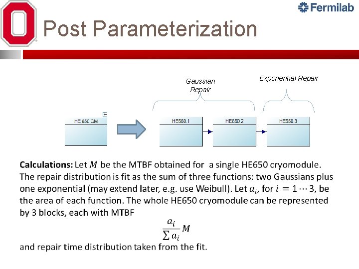
Post Parameterization Gaussian Repair Exponential Repair

Ion Source & LEBT System q q q The ion source/LEBT system is different from SNS. Filament type with higher MTBF, has online hot spares, no Cs, no RF source, and many other changes. Since the lifetime of the ion source is still very low (300 hours), a switching magnet switches to the hot spare as soon as one of the sources fails. The system is subdivided into two subsystems: Subsystem 1 : Two ion sources (1 is a hot spare) in parallel along with a solenoid, scanner and power supplies for each of them. Subsystem 2 Bending magnet and everything downstream, which do not have hot spares. Switching ion sources take ~10 minutes, and a tuning time of 2 hours. For those without hot spares, the system goes offline and the repair is ~10 hours. Ion Source

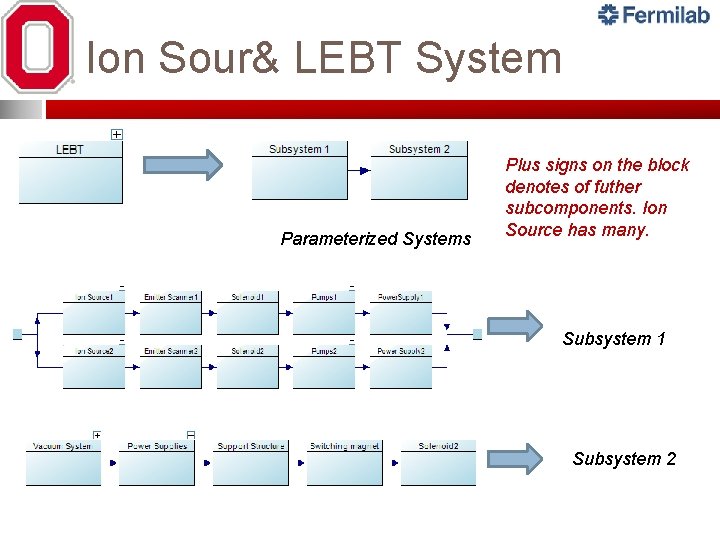
Ion Sour& LEBT System Parameterized Systems Plus signs on the block denotes of futher subcomponents. Ion Source has many. Subsystem 1 Subsystem 2

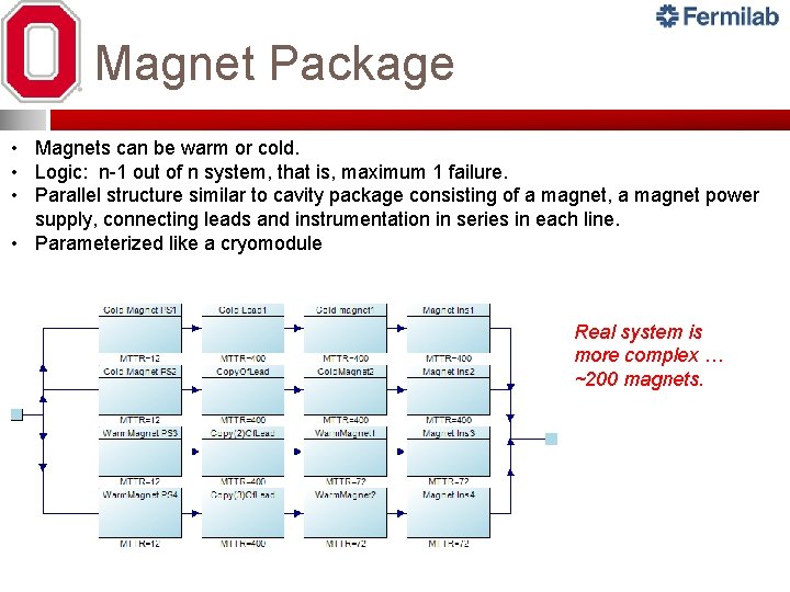
Magnet Package • Magnets can be warm or cold. • Logic: n-1 out of n system, that is, maximum 1 failure. • Parallel structure similar to cavity package consisting of a magnet, a magnet power supply, connecting leads and instrumentation in series in each line. • Parameterized like a cryomodule Real system is more complex … ~200 magnets.

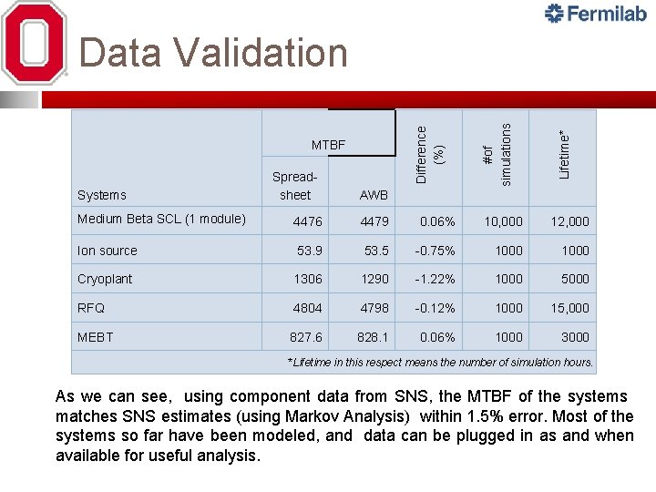
Systems Spreadsheet Lifetime* MTBF #of simulations Difference (%) Data Validation AWB Medium Beta SCL (1 module) 4476 4479 0. 06% 10, 000 12, 000 Ion source 53. 9 53. 5 -0. 75% 1000 Cryoplant 1306 1290 -1. 22% 1000 5000 RFQ 4804 4798 -0. 12% 1000 15, 000 MEBT 827. 6 828. 1 0. 06% 1000 3000 *Lifetime in this respect means the number of simulation hours. As we can see, using component data from SNS, the MTBF of the systems matches SNS estimates (using Markov Analysis) within 1. 5% error. Most of the systems so far have been modeled, and data can be plugged in as and when available for useful analysis.

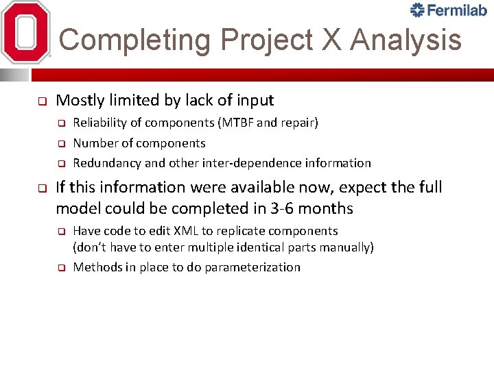
Completing Project X Analysis q Mostly limited by lack of input q q Reliability of components (MTBF and repair) Number of components Redundancy and other inter-dependence information If this information were available now, expect the full model could be completed in 3 -6 months q q Have code to edit XML to replicate components (don’t have to enter multiple identical parts manually) Methods in place to do parameterization

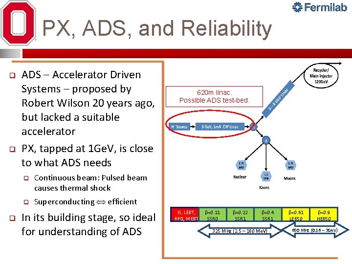
PX, ADS, and Reliability q q q ADS – Accelerator Driven Systems – proposed by Robert Wilson 20 years ago, but lacked a suitable accelerator PX, tapped at 1 Ge. V, is close to what ADS needs q Continuous beam: Pulsed beam causes thermal shock q Superconducting efficient In its building stage, so ideal for understanding of ADS 620 m linac. Possible ADS test-bed. IS, LEBT, RFQ, MEBT b=0. 11 SSR 0 b=0. 22 SSR 1 b=0. 4 SSR 1 325 MHz (2. 5 – 160 Me. V) b=0. 61 LE 650 b=0. 9 HE 650 MHz (0. 16 – 3 Ge. V )

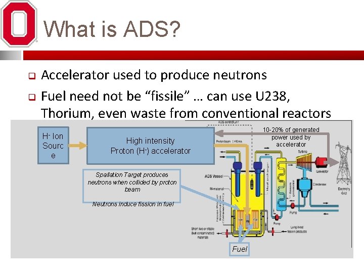
What is ADS? q q Accelerator used to produce neutrons Fuel need not be “fissile” … can use U 238, Thorium, even waste from conventional reactors H- Ion Sourc e 10 -20% of generated power used by accelerator High intensity Proton (H-) accelerator Spallation Target produces neutrons when collided by proton beam Neutrons induce fission in fuel Fuel

Importance of Reliability to ADS q More stringent for ADSS are and complex. q Availability >99% compared to <80% for the Tevatron q Maximum of 3‑ 5 failures a year compared to 70 -80 typical for existing accelerators q Reliability analysis exposes the weakness in the design – indispensable for ADS design. q Ion source fails often q Cryomodule repair is a major source of downtime. q Beam tuning is another major area of downtime.

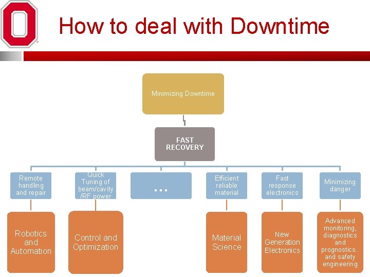
How to deal with Downtime Minimizing Downtime FAST RECOVERY Remote handling and repair Robotics and Automation Quick Tuning of beam/cavity /RF power Control and Optimization … Efficient reliable material Material Science Fast response electronics Minimizing danger New Generation Electronics Advanced monitoring, diagnostics and prognostics. . and safety engineering

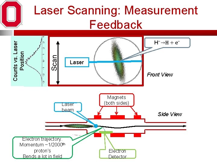
Beam Control & ADS q q Frequent beam interruptions leads to thermal shocks on the targets, leading to damage. Many “short” interruptions ok , longer ones should be limited to 3 -5 a year. q Definition of “short” depends on nature of fuel … seconds to minutes Present accelerators: ~80 medium to long failures a year q Tuning time ~hours – not feasible for ADS. q Intelligent controls can reduce this, increasing availability. ADS needs many improvements. Controls may not top the list … but it is also needed, and it is where I might contribute q

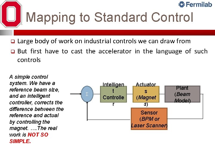
Mapping to Standard Control Large body of work on industrial controls we can draw from q But first have to cast the accelerator in the language of such controls q A simple control system. We have a reference beam size, and an intelligent controller, corrects the difference between the reference and actual by controlling the magnet. …. The real work is NOT SO SIMPLE. Σ Intelligen t Controlle r Actuator s (Magnet s) Sensor Ref Beam size (BPM or Laser Scanner) Plant (Beam Model)

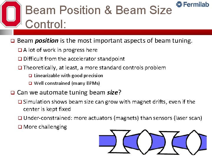
Beam Position & Beam Size Control: q Beam position is the most important aspects of beam tuning. q A lot of work in progress here q Difficult from the accelerator standpoint q Theoretically, at least, a more standard controls problem q q q Linearizable with good precision Well constrained (many BPMs) Can we automate tuning beam size? q Simulation shows beam size can grow with magnet drifts, even if the center is kept fixed q Under-constrained: more actuators (magnets) than sensors (laser scan) q More challenging

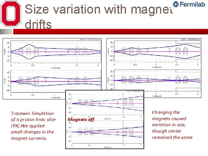
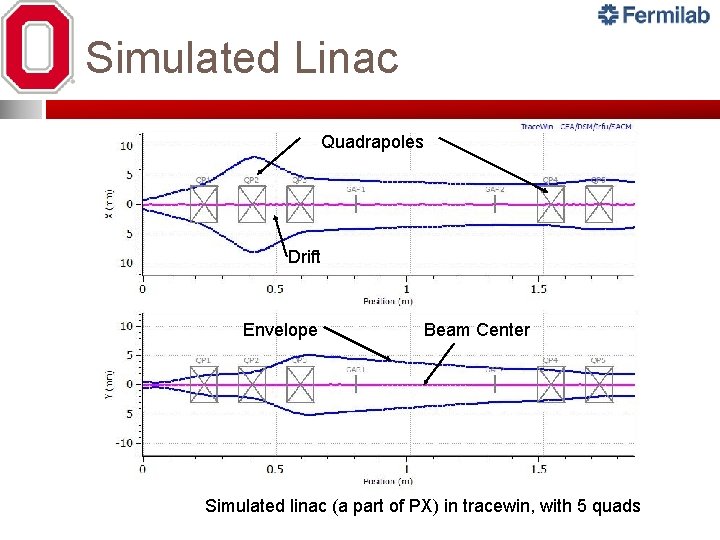
Size variation with magnet drifts Tracewin Simulation of a proton linac slice (PX). We applied small changes in the magnet currents. Magnets off Changing the magnets caused variation in size, though center remained the same

H⁻→H + e⁻ Scan Counts vs. Laser Position Laser Scanning: Measurement Feedback Laser Front View Laser beam Electron trajectory. Momentum ~1/2000 th proton’s Bends a lot in field Magnets (both sides) Side View Electron Detector

Beam Modeling q

Simulated Linac Quadrapoles Drift Envelope Beam Center Simulated linac (a part of PX) in tracewin, with 5 quads

Beam Modeling q

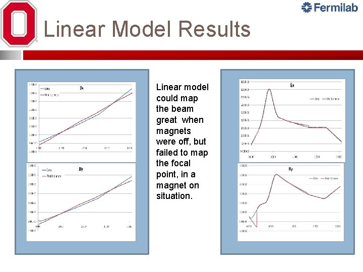
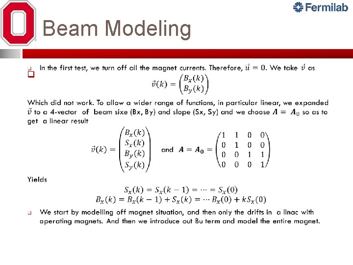
Linear Model Results Linear model could map the beam great when magnets were off, but failed to map the focal point, in a magnet on situation.

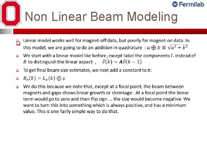
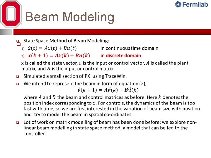
Non Linear Beam Modeling q

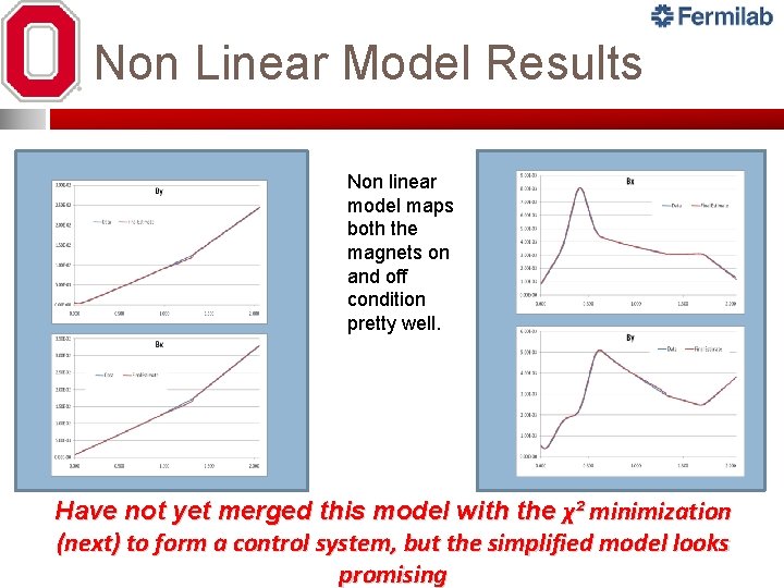
Non Linear Model Results Non linear model maps both the magnets on and off condition pretty well. Have not yet merged this model with the χ² minimization (next) to form a control system, but the simplified model looks promising

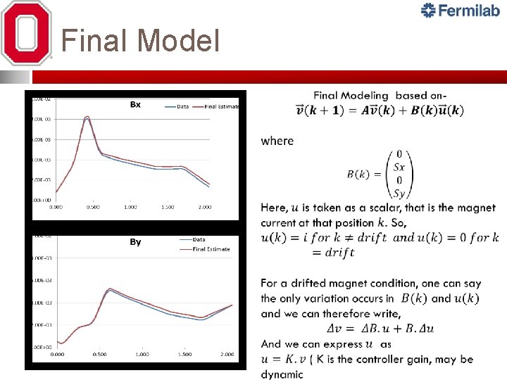
Final Model

χ2 Minimization Control Technique

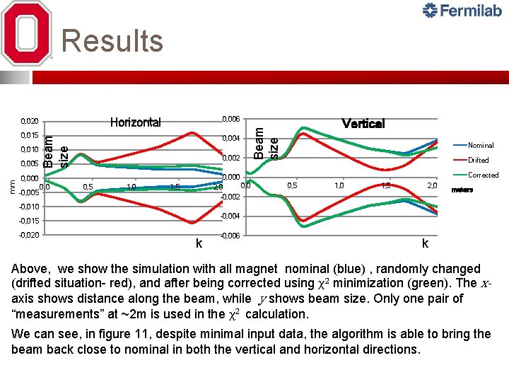
Results mm 0, 005 0, 002 0, 000 0, 0 2, 0 -0, 002 0, 000 -0, 005 0, 0 0, 5 1, 0 1, 5 Vertical Beam size 0, 010 0, 004 Beam size 0, 015 0, 006 Horizontal 0, 020 Nominal Drifted Corrected 0, 5 1, 0 1, 5 2, 0 meters -0, 010 -0, 004 -0, 015 -0, 020 k -0, 006 k Above, we show the simulation with all magnet nominal (blue) , randomly changed (drifted situation- red), and after being corrected using χ2 minimization (green). The xaxis shows distance along the beam, while y shows beam size. Only one pair of “measurements” at ~2 m is used in the χ2 calculation. We can see, in figure 11, despite minimal input data, the algorithm is able to bring the beam back close to nominal in both the vertical and horizontal directions.

Controls : what’s next? Beam profile control is a new area to explore We may be able to handle such under constrained problems q Merge the simplified beam model with χ2 minimization q q However, χ2 minimization is not common to control systems Try to overlay a 2 nd “state space” model with time (rather than position) as the variable See if conventional control methods can be applied More realistic simulations to see whether such solutions to under-constrained systems actually work

Acknowledgement My supervisors : Aseet Mukherjee, Jim Kerby, and Rama K Yedavalli. Steve Holmes, for giving me an opportunity to work in PX. And to everyone in TD and AD, as well as at CDF who has helped me gain understanding of accelerators and their components. George Dodson, ORNL, for his reliability data on SNS. Tom Himel, SLAC, for Avail. Sim.