RELATIVE FACTOR ABUNDANCE SVETLANA LEDYAEVA RICARDIAN MODEL RECALL

RELATIVE FACTOR ABUNDANCE SVETLANA LEDYAEVA

RICARDIAN MODEL RECALL Technological differences between countries are the classical driving force for international trade flows. Countries tend to export goods in which they have a comparative advantage. 2/16
 One")
ASSUMPTIONS OF THE RICARDIAN TECHNOLOGY MODEL • • Two countries (EU and Kenya) One factor of production (Labour) Two final goods (Food and Chemicals) Constant returns to scale production functions Perfect competition Labor is mobile between sectors, but not between countries Costless trade in final goods (no impediments to trade) Technology differs between countries Page 3

ASSUMPTIONS OF HECKSCHER-OHLIN MODEL • • • Two countries Two factors of production: Capital (K) & Labour (L) Two final goods (Good 1 more capital intensive) Constant returns to scale production functions Perfect competition Labor is mobile between sectors, but not between countries Costless trade in final goods (no impediments to trade) Identical production technology in the two countries: F(K, L) Identical homothetic tastes in the two countries Countries differ in their (relative) factor endowments Page 4

INTUITIONS OF H-O MODEL In Autarky • Relatively large supply of K • Low relative price of K • Cheap to produce K-intensive good • “Comparative advantage” in K-intensive good Open up for trade • Export K-intensive good Page 5

OUTLINE • Basic setup • Factor price equalization and Stolper–Samuelson theorem • Rybczynski theorem • Heckscher-Ohlin theorem • Empirical evidence
 • Let K and L denote")
BASIC SETUP Firm’s input choices (for any good) • Let K and L denote some combination of capital and labor that produce one unit of output F (K, L) = 1 • Profits associated with this input combination are π(1)=p. F (K, L) – r. K – w. L =p – r. K – w. L • CRS: output Q can be produced with QK and QL • Profits at any scale of operations Q: π(Q)=p. Q – r. QK – w. QL = Qπ(1) • Thus, we only need to study how input requirements for unit production, K & L, are determined

BASIC SETUP Capital • Isoquant: different Q=1 combinations of K & L that produce the same output Q • F(K, L) determines the shape of isoquants normally bowed inward Isoquant Slope Diminishing Marginal Rate of Substitution Q=0. 7 Labour

BASIC SETUP Capital • Production costs c = r. K + w. L pe slo = • Isocost: different -w /r combinations of K & L that incur the same cost Isocost • Straight line slope = -(w/r) Labour

BASIC SETUP Capital • Firm max profit choose K M=1 & L along the unit isoquant to min cost pe slo = -w /r • Solution: when unit isoquant K is tangent to isocost A • At point A: Slope of isoquant = slope of isocost = -(w/r) L Labour

FACTOR PRICE EQUALIZATION • Hence, optimal input choices are determined by factor prices • Next question: how are factor prices determined? • We show in the following Lerner diagram

FACTOR PRICE EQUALIZATION Capital Q=1/p • unit value isoquant = input needed to produce one unit of value • shows different combinations of K & L to produce the same amount of output, 1/p Labor

FACTOR PRICE EQUALIZATION Capital • unit value isocost line = input 1/r 0 combinations leading to one unit value of costs slo pe = /r 0 -w 1/r 1 • w L + r. K = 1 • An increase in the cost of slo pe = capital from r 0 to r 1 rotates the -w unit value isocost line inwards /r 1 1/w Labour

FACTOR PRICE EQUALIZATION Capital Q=1/p • Recall that perfect competition assumption implies zero profit 1/r • The isocost line must be A tangent to the isoquant Labour 1/w

FACTOR PRICE EQUALIZATION Capital Q 1=1/p 1 • In the case of 2 goods (1, 2) , assume good 1 is more Q 2=1/p 2 capital intensive • If both goods are produced 1/r the isocost line must be tangent to both isoquants A • Hence, goods prices uniquely determine factor prices B Labour 1/w
 & 2 goods")
FACTOR PRICE EQUALIZATION In the case of 2 countries (A, B) & 2 goods (1, 2) • Trade equalizes good prices: P 1 A=P 1 B & P 2 A=P 2 B • Thus, WA = W B & R A = R B • This is the factor price equalization (FPE).

STOLPER-SAMUELSON THEOREM • We have shown good prices factor prices • What happen to factor prices when good prices changes?

STOLPER-SAMUELSON THEOREM Capital Q 1=1/p 1 • Recall: good 1 is capital intensive and good 2 is labor Q 2=1/p 2 intensive • If p 1 , then Q 1=1/p 1 1/r • Unit value isoquant curve shifts inward X Y Labour 1/w

STOLPER-SAMUELSON THEOREM Capital Q 1=1/p 1 • When price of good 1 increases Q 2=1/p 2 • The new isoquants determines the new tangent 1/r isocost line • 1/r , so r ; reward to A capital (used intensively in 1/r’ good 1) rises A’ B Labor • 1/w , so w ; reward to B’ 1/w labor falls 1/w’

STOLPER-SAMUELSON THEOREM • We have shown that an increase in the price of capital intensive good (good 1) increases returns to capital (rent) & decreases returns to labor (wage) • Similarly, we can show if the price of labor intensive good (good 2) rises, wage increases and rent decreases • Taken together this is the Stolper-Samuelson theorem

RYBCZYNSKI THEOREM • We have shown good prices determine factor prices, which then determine input choices: p r, w K*, L* • Given these parameters, how to allocate K & L between the production of each good, i. e. q 1 vs q 2? • We use PPF (all possible combination of q 1 & q 2 given fixed total resources)

RYBCZYNSKI THEOREM q 2 • Imperfect substitution of inputs slope = - p 1/p 2 PPF bowed outward • Iso-revenue line shows all combinations of q 1 & q 2 that give us the same revenue: Iso-revenue line q 2 * p 1 q 1 + p 2 q 2 = REV • To max revenue, iso-revenue is tangent to PPF • Optimal output choices: q 1* & q 2 * PPF q 1 * q 1 PPF slope – marginal rate of transformation

RYBCZYNSKI THEOREM q 2 • What happens when total resource stock changes? • For example, if total K increases, PPF shifts outward • Good 1 is capital intensive PPF intercept for good 1 shifts capital Rybczynski line more • New PPF tangent to new isorevenue line • q 1* , q 2* q 1

RYBCZYNSKI THEOREM • Given final goods prices, an increase in the capital stock increases the production of good 1(uses capital intensively) and reduces the production of good 2(uses labour intensively) • Similarly: increase in labour raises good 2 production & lowers good 1 production • Together: Rybczynski theorem

HECKSCHER-OHLIN THEOREM • Till now, we have only discussed production decisions, or Supply q 2 Income/revenue line • Given prices of 2 goods, max revenue/income at tangent point A A ppf q 1 • Let’s bring in Demand to pin down the equilibrium under Autarky and Trade

HECKSCHER-OHLIN THEOREM q 2 • Given income and good prices, consumer chooses q 1 d, q 2 d to max utility • Iso-utility curve tangent to q 2 B d revenue/income line U=2 Revenue/income line slope = - p 1/p 2 U=1 q 1 d q 1

HECKSCHER-OHLIN THEOREM q 2 • In Autarky, supply = demand Uau • Good prices adjust to ensure point A = point B A B income lineau ppf q 1
 share the same technology")
HECKSCHER-OHLIN THEOREM • In H-O model, 2 countries (A, B) share the same technology and preferences (iso-utility curve) • The only difference is factor abundance • Assume A is relatively capital abundant and B is relatively labour abundant • Country A is capable of producing more capital intensive good (good 1) and country B is capable of producing more labor intensive good (good 2) Different PPF shape

UA q 2 UB slope = - p 1 A/p 2 A slope = - p 1 B/p 2 B ppf. A q 1

HECKSCHER-OHLIN THEOREM In autarky: • K-intensive country A produces more K-intensive good 1; Lintensive country B produces more L-intensive good 2 • p 2 A/p 1 A < p 2 B/p 1 B K-intensive good 1 is relatively cheap in K-intensive country A With free trade: • Free trade equalized prices; suppose the trade price lies between the 2 autarky price ratios

UA q 2 UB prod. B slope = - p 2 A/p 1 A con. B con. A prod. A slope = - p 2 B/p 1 B ppf. A q 1

HECKSCHER-OHLIN THEOREM With free trade: • K-abundant country A export K-intensive good 1 • L-abundant country B export L-intensive good 2 • Both countries gain from trade Heckscher-Ohlin theorem • Under free trade a country exports the good that uses the relatively abundant factor of production relatively intensively

EMPIRICAL EVIDENCE • The H-O model is probably the most influential model in all of Trade. So how do we assess how useful it is in a description of the real world? Challenge: • H-O theorem: 2 goods & 2 factors • In reality: likely to have more goods than factors • Solution: compare “factor content” rather than “good content” in trade flow
: 2 inputs K & L;")
EMPIRICAL EVIDENCE Tests on US data • Leontief (1953): 2 inputs K & L; compute the K/L ratio of US imports/exports in 1947; - exports: $13, 700 per worker - imports: $18, 200 per worker • US exports were less capital-intensive than US imports, even though the US is the most capital-abundant country in the world: Leontief paradox.
 tested")
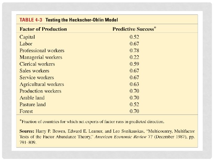
EMPIRICAL EVIDENCE Tests on global data • Bowen, Leamer, and Sveikauskas (1987, AER) tested the Heckscher-Ohlin model on data from 27 countries and 12 factors. • Confirmed the Leontief paradox on an international level.

EMPIRICAL EVIDENCE Why lack of empirical evidence? • Heckscher-Ohlin model predicts that free trade will generate enough trade flow to equalize factor prices across trading countries • But because factor prices are not equalized across countries: missing trade (Daniel Trefler 1995, AER) • Reason: assumption of identical technology among countries may be wrong. - Technology affects the productivity of labor and therefore the value of labor services. A country with high technology and a high value of labor services would not necessarily import a lot from a country with low technology and a low value of labor services
 relaxes the identical")
EMPIRICAL EVIDENCE Why lack of empirical evidence? • Daniel Trefler (1995) relaxes the identical technology assumptions to fit the reality • Also adjust the preferences assumptions: for example, allow consumer to prefer home goods to foreign goods • Sign test results improved considerably (nearly perfectly accurate)

CONCLUSION • Country exports the good that uses the relatively abundant factor of production relatively intensively • Lack of empirical evidence supporting simple 2 factor & 2 goods model, which does not fit reality • Model predicts better with adjustments

AREAS FOR FUTURE WORK • With trade costs? • Empirical H-O with endogenous technology? (e. g. Skillbiased technological change. ) Traditional H-O theory takes resources as orthogonal to technology. • Endowments are not exogenous either. K and L are likely to respond to technological differences. (A “dynamic H-O model”. )
- Slides: 40