Relationships in Categorical Data with Intro to Probability

Relationships in Categorical Data with Intro to Probability Concepts in Statistics

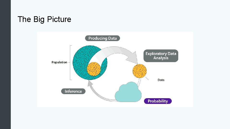
The Big Picture

Variables Recall the difference between quantitative and categorical variables: • • Quantitative variables have numeric values that can be averaged. A quantitative variable is frequently a measurement – for example, a person’s height in inches. Categorical variables are variables that can have one of a limited number of values, or labels. Values that can be represented by categorical variables include, for example, a person’s eye color, gender, or home state; a vehicle’s body style (sedan, SUV, minivan, etc. ); a dog’s breed (bulldog, greyhound, beagle, etc. ).

Two-way Tables As we organize and analyze data from two categorical variables, we make extensive use of two-way tables. Two-way tables for two categorical variables are in some ways like scatterplots for two quantitative variables: they give us a useful snapshot of all of the data organized in terms of the two variables of interest. This will be helpful in finding and comparing patterns.

Categorical Variables The relationship between two categorical variables may be summarized using both • Two-way tables: compactly summarizes totals across the groups. • Conditional percentages: shows the proportions over all the values of the explanatory variable. Conditional percentages are calculated separately for each value of the explanatory variable. When we try to understand the relationship between two categorical variables, we compare the distributions of the response variable for values of the explanatory variable. In particular, we look at how the pattern of conditional percentages differs between the values of the explanatory variable.

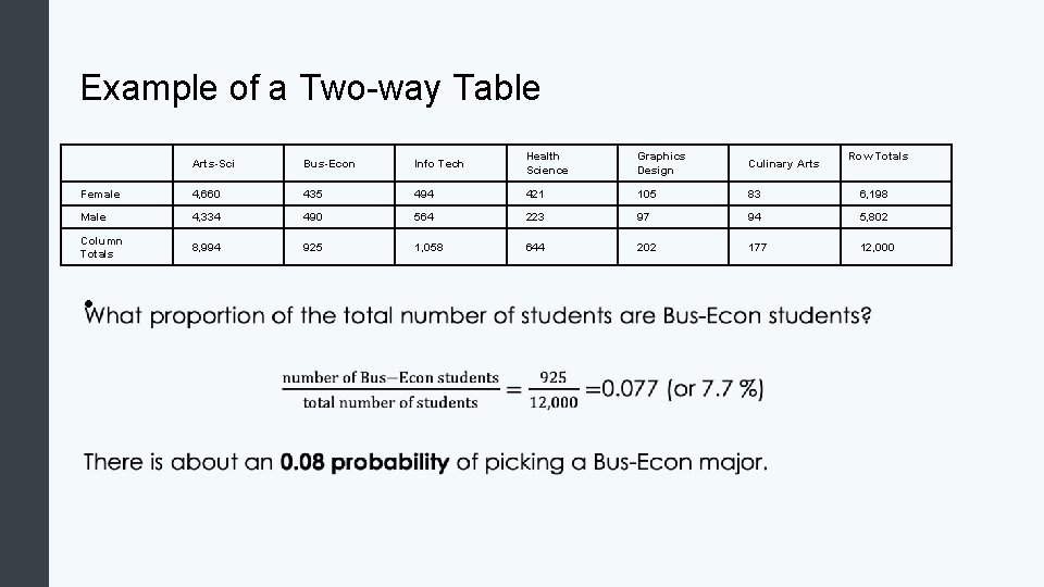
Example of a Two-way Table Row Totals Arts-Sci Bus-Econ Info Tech Health Science Graphics Design Culinary Arts Female 4, 660 435 494 421 105 83 6, 198 Male 4, 334 490 564 223 97 94 5, 802 Column Totals 8, 994 925 1, 058 644 202 177 12, 000 •

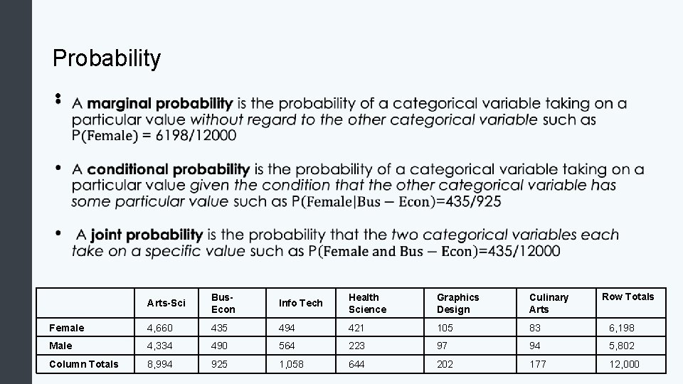
Probability • Row Totals Arts-Sci Bus. Econ Info Tech Health Science Graphics Design Culinary Arts Female 4, 660 435 494 421 105 83 6, 198 Male 4, 334 490 564 223 97 94 5, 802 Column Totals 8, 994 925 1, 058 644 202 177 12, 000

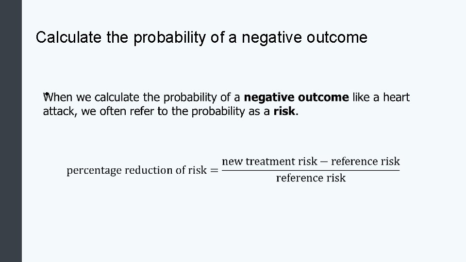
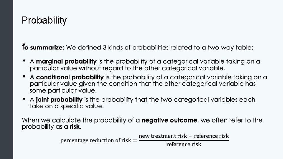
Calculate the probability of a negative outcome •

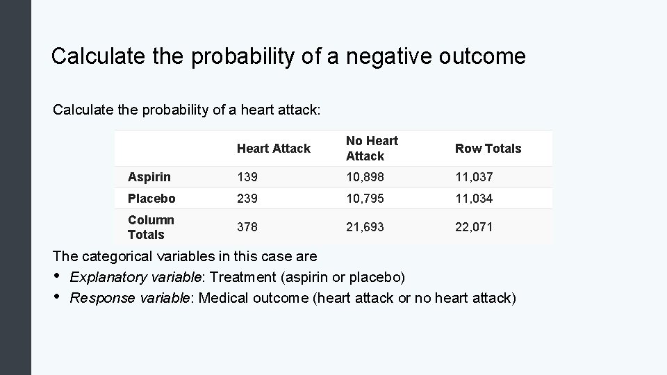
Calculate the probability of a negative outcome Calculate the probability of a heart attack: Heart Attack No Heart Attack Row Totals Aspirin 139 10, 898 11, 037 Placebo 239 10, 795 11, 034 Column Totals 378 21, 693 22, 071 The categorical variables in this case are • Explanatory variable: Treatment (aspirin or placebo) • Response variable: Medical outcome (heart attack or no heart attack)

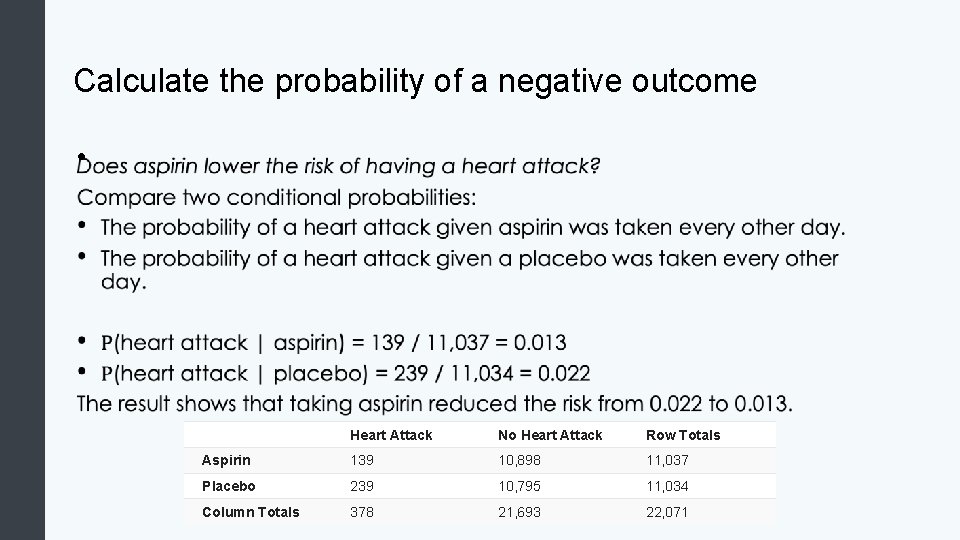
Calculate the probability of a negative outcome • Heart Attack No Heart Attack Row Totals Aspirin 139 10, 898 11, 037 Placebo 239 10, 795 11, 034 Column Totals 378 21, 693 22, 071

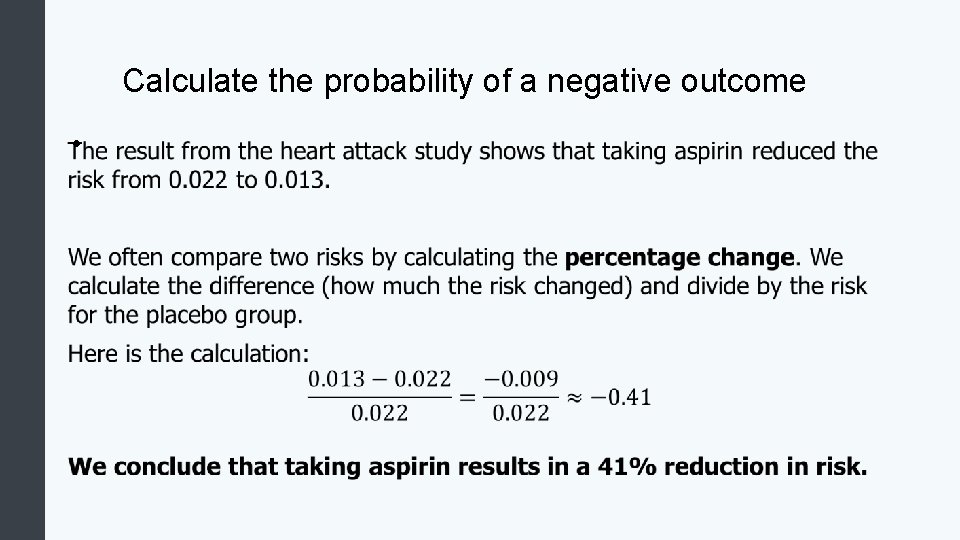
Calculate the probability of a negative outcome •

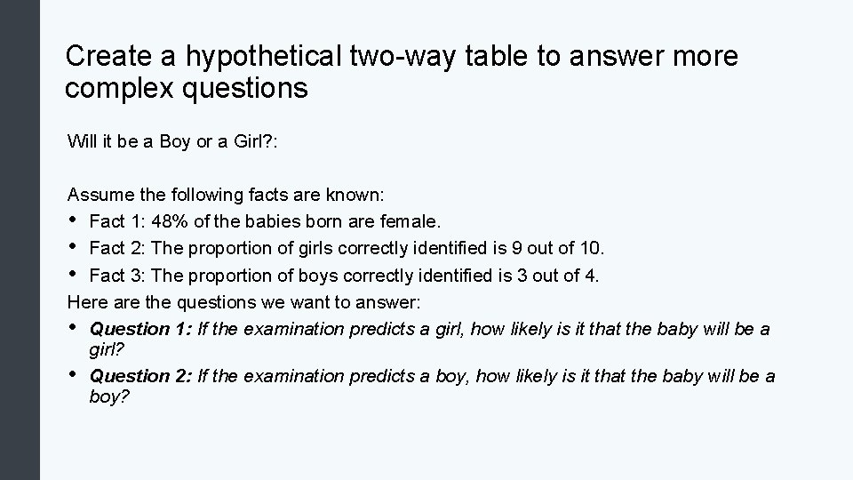
Create a hypothetical two-way table to answer more complex questions Will it be a Boy or a Girl? : Assume the following facts are known: • Fact 1: 48% of the babies born are female. • Fact 2: The proportion of girls correctly identified is 9 out of 10. • Fact 3: The proportion of boys correctly identified is 3 out of 4. Here are the questions we want to answer: • Question 1: If the examination predicts a girl, how likely is it that the baby will be a girl? • Question 2: If the examination predicts a boy, how likely is it that the baby will be a boy?

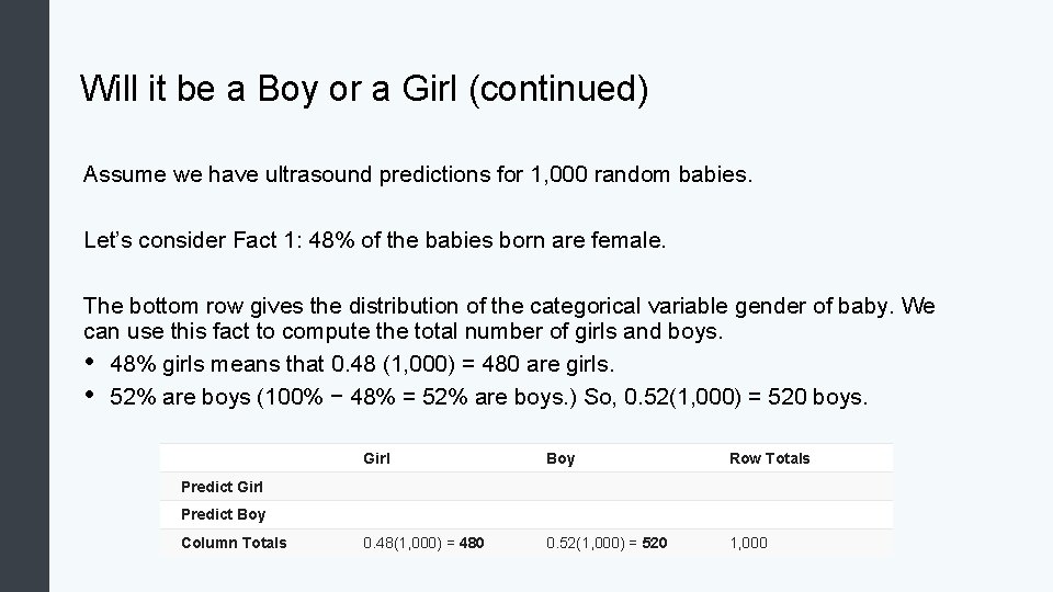
Will it be a Boy or a Girl (continued) Assume we have ultrasound predictions for 1, 000 random babies. Let’s consider Fact 1: 48% of the babies born are female. The bottom row gives the distribution of the categorical variable gender of baby. We can use this fact to compute the total number of girls and boys. • 48% girls means that 0. 48 (1, 000) = 480 are girls. • 52% are boys (100% − 48% = 52% are boys. ) So, 0. 52(1, 000) = 520 boys. Girl Boy Row Totals 0. 48(1, 000) = 480 0. 52(1, 000) = 520 1, 000 Predict Girl Predict Boy Column Totals

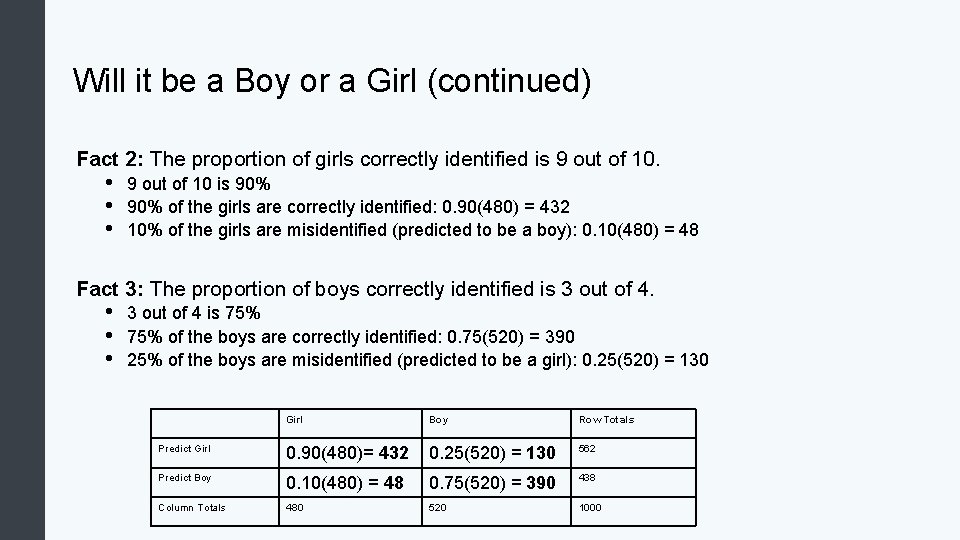
Will it be a Boy or a Girl (continued) Fact 2: The proportion of girls correctly identified is 9 out of 10. • • • 9 out of 10 is 90% of the girls are correctly identified: 0. 90(480) = 432 10% of the girls are misidentified (predicted to be a boy): 0. 10(480) = 48 Fact 3: The proportion of boys correctly identified is 3 out of 4. • • • 3 out of 4 is 75% of the boys are correctly identified: 0. 75(520) = 390 25% of the boys are misidentified (predicted to be a girl): 0. 25(520) = 130 Girl Boy Row Totals Predict Girl 0. 90(480)= 432 0. 25(520) = 130 562 Predict Boy 0. 10(480) = 48 0. 75(520) = 390 438 Column Totals 480 520 1000

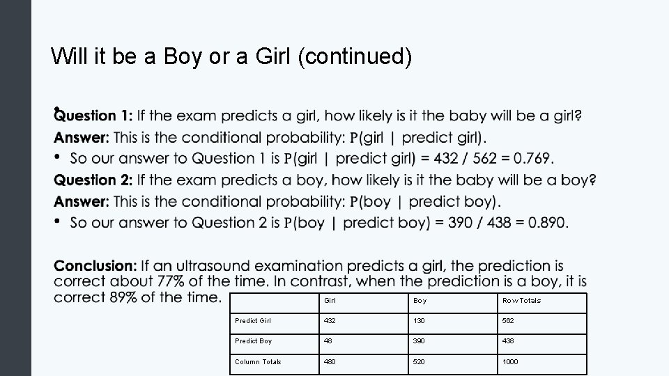
Will it be a Boy or a Girl (continued) • Girl Boy Row Totals Predict Girl 432 130 562 Predict Boy 48 390 438 Column Totals 480 520 1000

Probability •

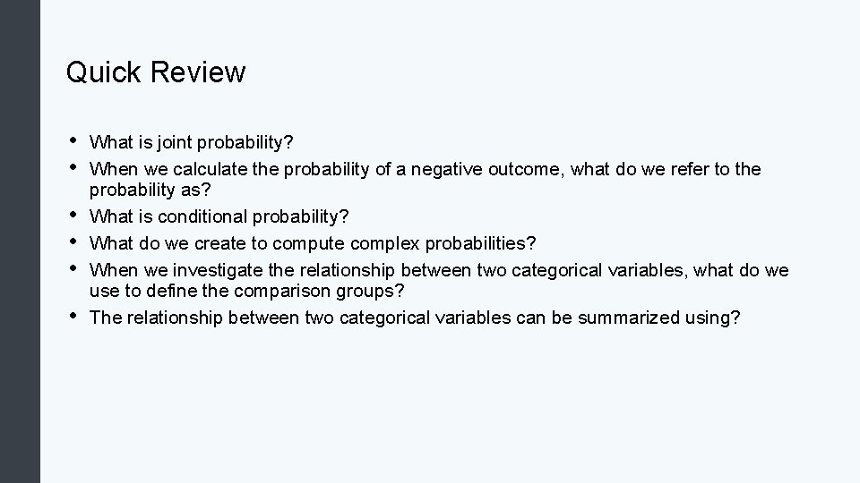
Quick Review • • • What is joint probability? When we calculate the probability of a negative outcome, what do we refer to the probability as? What is conditional probability? What do we create to compute complex probabilities? When we investigate the relationship between two categorical variables, what do we use to define the comparison groups? The relationship between two categorical variables can be summarized using?