Relationship Between Quantitative Data Regression and Correlation Analysis

Relationship Between Quantitative Data (Regression and Correlation Analysis)

One-dimensional Statistics – we assess 1 variable (statistical character) in different sets of data (samples, populations); we analyse differences between 2 sets of data (methods: statistical tests) 2 -dimensional Statistics – we assess 2 variables in 1 set of data; we try to qualify and describe relationship between 2 variables, one being an independent and one being a dependent var. predicted by the independent v. (methods: regression and correlation analyses)

Relationships between 2 variables: - functional - statistical (correlative) 1. Functional Relationship 2. (Mathematics, Physics) 3. - the magnitude of dependent variable is determined by the magnitude of independent variable: each value of the independent variable (xi) corresponds to 1 exact value of the dependent variable ( yi) Description: exact equation (formula) e. g. circle radius (r) and circumference (y=2 r)

Graphical description: circle radius (r) and circumference (y=2 r) yi (2 r) (dependent v. - „outcome“) Strictly causal relationship - not affected by random xi (r) (independent v. - „input“)

2. Statistical Relationship (Correlative) 3. (Biology) - free relation: the magnitude of one of the variables probably changes as the magnitude of the second variable changes. Each value of xi corresponds to several random values of yi and also the reverse is possible (In such case it is not resonable to consider there is an independent and dependent variable e. g. fore- and hindleg lengths in animals, human height and weight …).

Graphical description: to display the data points (each point has its values in both axes: xi, yi - correlation pair) yi (Weight) (Correlation Chart, Scatter Diagram) xi (Height)

Different pattern of scatter charts different types of relationships A – Relationship between two data sets exists (tight direct relation) B – Relationship among the two data sets exists (tight inverse relation) C – Evidence of poor or no significant relation

Description of correlative relationship: To estimate the best-fit function that can express the relationship and to determine its equation (approximation -> smooth diagram). According to the pattern of scatter diagram : a) linear correlative relation b) non-linear correlative relation

A) Linear Correlative Relation 1. Empirical curve (describes the relation in a sample set) - when we have several equal values xi several values yi mean. Join the means = empirical curve (estimation of the best-fit linear function) yi (Weight) (empirical curve) xi (Height)

2. Theoretical regression line (describes the relation in a population) y=a+bx Method: regression analysis (linear regression) Characteristics of the line: a (intercept) – represents the intercept point on axis y b (slope) = tg +a +b -a -b

Linear Regression (computes the parameters of the function: y= a+bx) Sample: n - number of members correlation pairs (xi ; yi)

2 points for the construction of the regression line: - we choose any x 1 y 1 = a + bx 1 - we choose any x 2 y 2 = a + bx 2 yi y 2 (Theoretical regression line) y 1 x 2 xi

3. Correlation Analysis – determines the level of association of X and Y (closeness of the relation) Correlation coefficient: r – quantitative expression of interaction force between X and Y (cluster of points around the line in scatter diagram – may be free or close).

r = -1; +1 r=0 No correlation r >0 r <0 Close direct c. Close inverse c. (X, Y increase together) X increases, Y decreases r =+1 r = -1 Functional direct r. Functional inverse r.

Significance of the Correlation Coefficient The correlation coefficient r is only an estimate of an actual cor. coef. in the population (denoted ). Is there (in fact) any correlation in the population? - We test the hypothesis of the independence (H 0: =0) using t-test: Test statistic: = n-2 SD of the correlation coef. : If t t ( ) H 0 is not true, correlation between X, Y really exists (r is significant) If t t ( ) H 0 is true, correlation between X, Y really does not exist (r is insignificant)

B) Non-linear Correlative Relation Scattered diagram: Difficulties in non-linear regression equations computer: polynomial regression different regression models (curves) E. g. The most common - quadratic : y=a+b 1 x+b 2 x 2 (second-order polynom)calculation of coefficients a, b 1, b 2.

Another method for the analysis of a non-linear relation is: Spearman Rank Correlation Ø Non-parametric method: used if either or both data (dependent or independent variables) are skewed (non-normal) Ø Can be used more generally then „parametric“ correl. coef. (in both linear and non-linear correlation), but is not as precise Ø Ranks of the measurements only are used in calculation (instead of observed values xi, yi) Sample: n- number of members correlation pairs (xi ; yi)

Variable X and Y is arranged separately: x 2 <x 4 <x 1 <x 5 <x 3 <x 8 <x 6 <x 7………. . 1 2 3 4 5 6 7 8 n y 3 <y 1 <y 5 <y 2 <y 4 <y 8 <y 7 <y 9………. . 1 2 3 4 5 6 7 8 n Di – difference between xi, yi ranks (D 1=3 -2, D 2=1 -4, D 3=5 -1 …) r. Sp = -1; +1 |r. Sp| > r( , n) significant correlation between X and Y |r. Sp| r( , n) insignificant correlation between X and Y

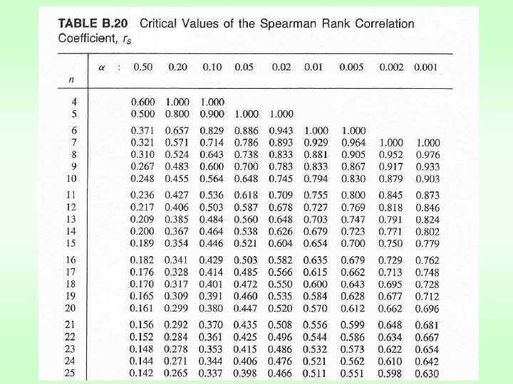
Example: The Spearman rank correlation coefficient, computed for the relation between wing and tail lengths among birds of a particular species :

Wing l. Rank No (X) of X 1 10. 2(cm) 1. 5 2 10. 2 1. 5 3 10. 3 3 4 10. 4 4 5 10. 5 5 6 10. 6 6 7 10. 7 7 8 10. 8 8. 5 9 10. 8 8. 5 10 11. 1 10 11 11. 2 11 12 11. 4 12 n=12 Tail l. (Y) 7. 1(cm) 7. 2 7. 4 7. 2 7. 8 7. 4 7. 6 7. 8 7. 9 7. 7 8. 3 Rank of Y 1 2. 5 5 5 2. 5 9. 5 5 7 9. 5 11 8 12 Di 0. 5 -1 -2 -1 2. 5 -3. 5 2 1. 5 -1 -1 3 0 D i 2 0. 25 1 4 1 6. 25 12. 25 4 2. 25 1 1 9 0 Di 2=42. 00 Crit. r. Sp (0. 01, 12)=0. 727 correlation between wing and tail lengths is statistically highly significant (really exists in the population).