Relational Query Optimization Chapter 15 1 Query Blocks

Relational Query Optimization Chapter 15 1

Query Blocks: Units of Optimization v An SQL query is parsed into a collection of query blocks : § An SQL query with no nesting and exactly one SELECT, FROM, WHERE, GROUP BY, and HAVING clause. § WHERE is in conjunctive normal form. 2

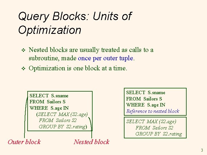
Query Blocks: Units of Optimization v v Nested blocks are usually treated as calls to a subroutine, made once per outer tuple. Optimization is one block at a time. SELECT S. sname FROM Sailors S WHERE S. age IN (SELECT MAX (S 2. age) FROM Sailors S 2 GROUP BY S 2. rating) Outer block SELECT S. sname FROM Sailors S WHERE S. age IN Reference to nested block SELECT MAX (S 2. age) FROM Sailors S 2 GROUP BY S 2. rating Nested block 3

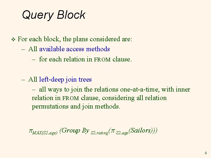
Query Block v For each block, the plans considered are: – All available access methods – for each relation in FROM clause. – All left-deep join trees – all ways to join the relations one-at-a-time, with inner relation in FROM clause, considering all relation permutations and join methods. MAX(S 2. age) (Group By S 2. rating( S 2. age(Sailors))) 4

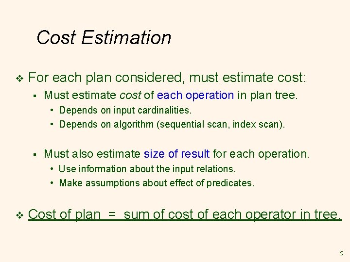
Cost Estimation v For each plan considered, must estimate cost: § Must estimate cost of each operation in plan tree. • Depends on input cardinalities. • Depends on algorithm (sequential scan, index scan). § Must also estimate size of result for each operation. • Use information about the input relations. • Make assumptions about effect of predicates. v Cost of plan = sum of cost of each operator in tree. 5

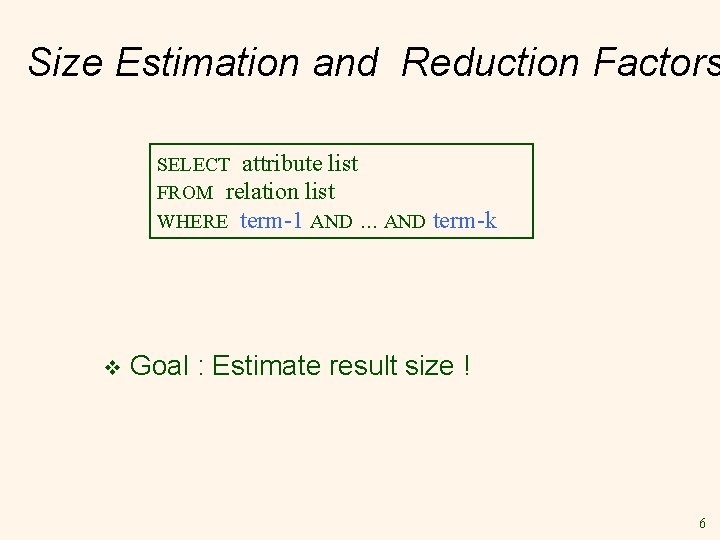
Size Estimation and Reduction Factors SELECT attribute list FROM relation list WHERE term-1 AND. . . AND v term-k Goal : Estimate result size ! 6

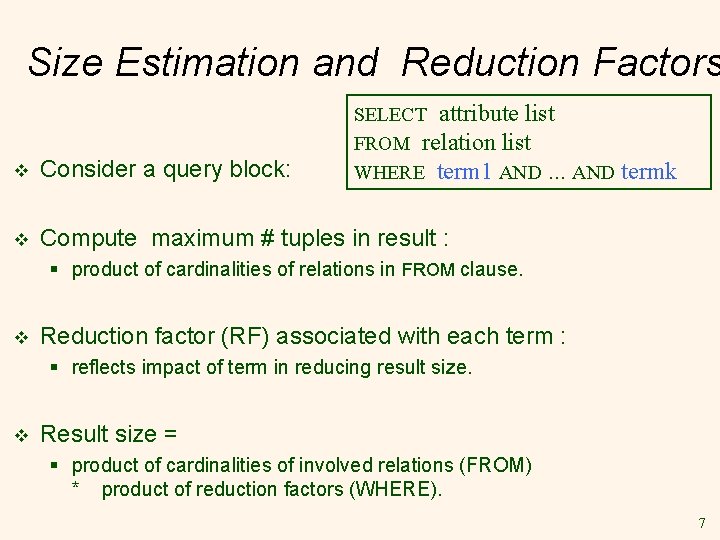
Size Estimation and Reduction Factors SELECT attribute list FROM relation list WHERE term 1 AND. . . AND v Consider a query block: v Compute maximum # tuples in result : termk § product of cardinalities of relations in FROM clause. v Reduction factor (RF) associated with each term : § reflects impact of term in reducing result size. v Result size = § product of cardinalities of involved relations (FROM) * product of reduction factors (WHERE). 7

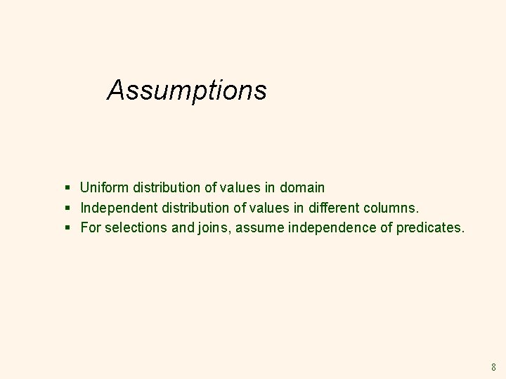
Assumptions § Uniform distribution of values in domain § Independent distribution of values in different columns. § For selections and joins, assume independence of predicates. 8

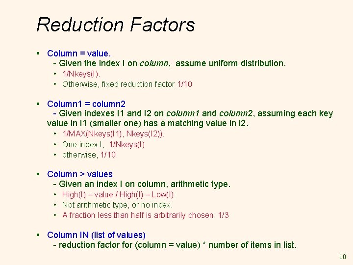
Reduction Factors § Column = value. - Given the index I on column, assume uniform distribution. • 1/Nkeys(I). • Otherwise, fixed reduction factor 1/10 § Column 1 = column 2 - Given indexes I 1 and I 2 on column 1 and column 2, assuming each key value in I 1 (smaller one) has a matching value in I 2. • 1/MAX(Nkeys(I 1), Nkeys(I 2)). • One index I, 1/Nkeys(I) • otherwise, 1/10 § Column > values - Given an index I on column, arithmetic type. • High(I) – value / High(I) – Low(I). • Not arithmetic type, or no index. • A fraction less than half is arbitrarily chosen: 1/3 § Column IN (list of values) - reduction factor for (column = value) * number of items in list. 10

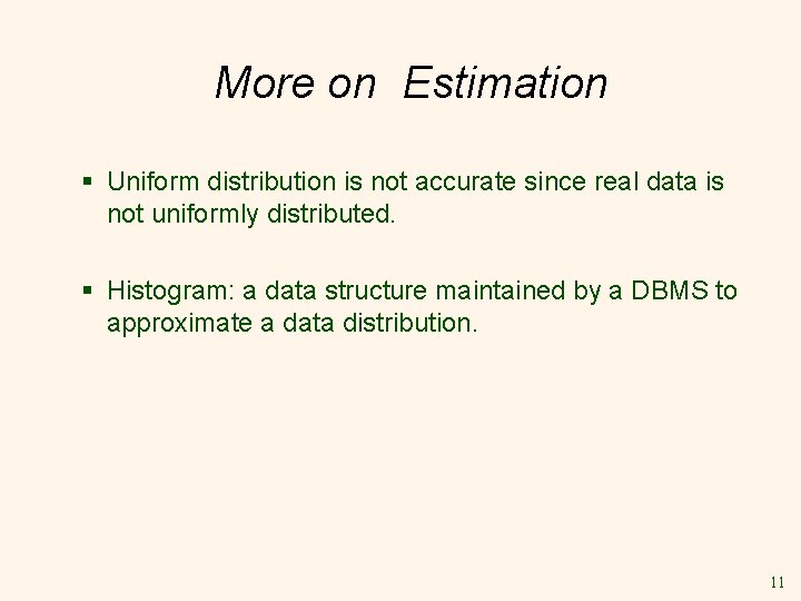
More on Estimation § Uniform distribution is not accurate since real data is not uniformly distributed. § Histogram: a data structure maintained by a DBMS to approximate a data distribution. 11

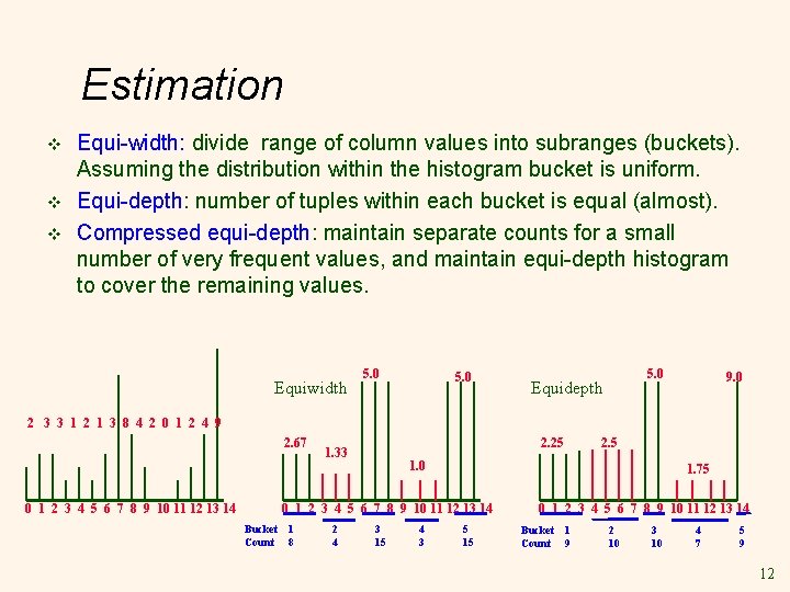
Estimation v v v Equi-width: divide range of column values into subranges (buckets). Assuming the distribution within the histogram bucket is uniform. Equi-depth: number of tuples within each bucket is equal (almost). Compressed equi-depth: maintain separate counts for a small number of very frequent values, and maintain equi-depth histogram to cover the remaining values. Equiwidth 5. 0 Equidepth 9. 0 2 3 3 1 2 1 3 8 4 2 0 1 2 4 9 2. 67 0 1 2 3 4 5 6 7 8 9 10 11 12 13 14 2. 25 1. 33 1. 0 1. 75 0 1 2 3 4 5 6 7 8 9 10 11 12 13 14 Bucket 1 Count 8 2 4 2. 5 3 15 4 3 5 15 0 1 2 3 4 5 6 7 8 9 10 11 12 13 14 Bucket 1 Count 9 2 10 3 10 4 7 5 9 12

Relational Algebra Equivalences v Allow us to choose different join orders v Allow us to `push’ selections and projections ahead of joins. 13

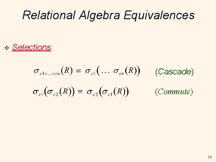
Relational Algebra Equivalences v Selections: (Cascade) (Commute) 14

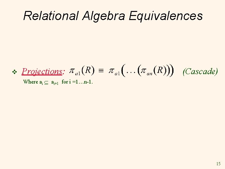
Relational Algebra Equivalences v Projections: (Cascade) Where ai ai+1 for i =1…n-1. 15

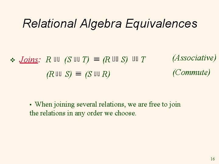
Relational Algebra Equivalences v Joins: R (R (S T) (R S) (S R) S) T (Associative) (Commute) • When joining several relations, we are free to join the relations in any order we choose. 16

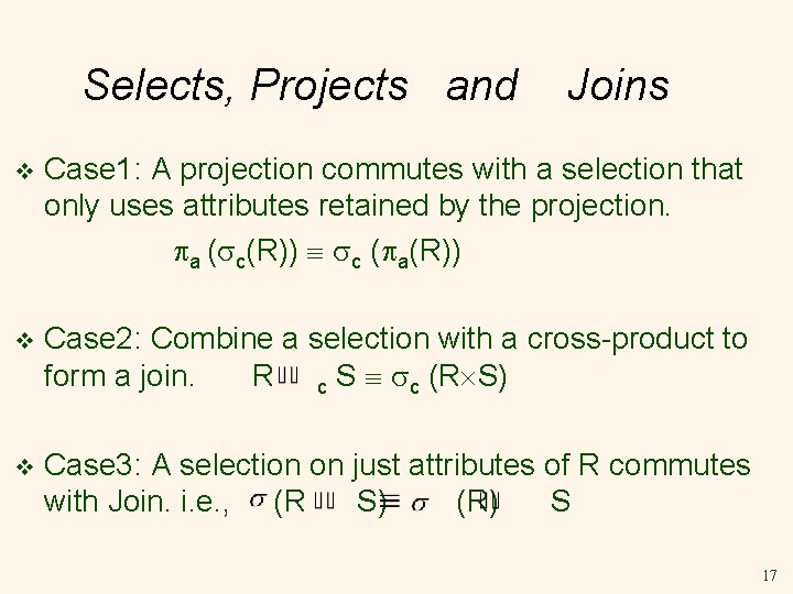
Selects, Projects and Joins v Case 1: A projection commutes with a selection that only uses attributes retained by the projection. a ( c(R)) c ( a(R)) v Case 2: Combine a selection with a cross-product to form a join. R c S c (R S) v Case 3: A selection on just attributes of R commutes with Join. i. e. , (R S) (R) S 17

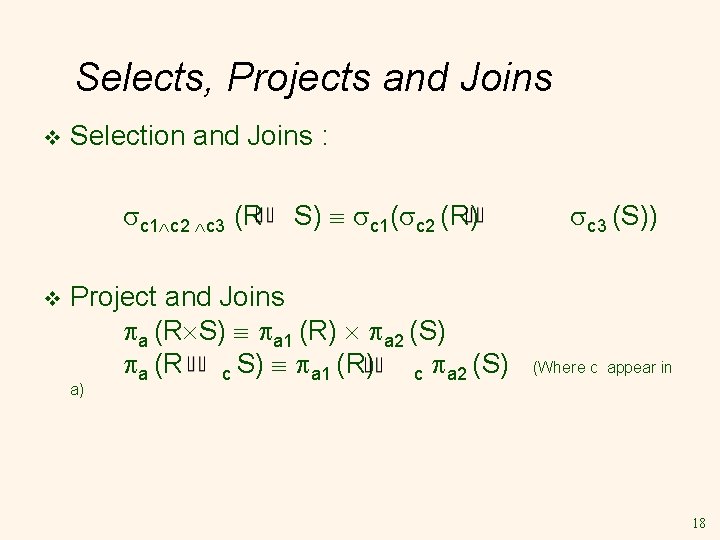
Selects, Projects and Joins v Selection and Joins : c 1 c 2 c 3 (R v S) c 1( c 2 (R) Project and Joins a (R S) a 1 (R) a 2 (S) a (R c S) a 1 (R) c a 2 (S) c 3 (S)) (Where c appear in a) 18

Enumeration of Alternative Plans v There are two main cases: § § Single-relation plans Multiple-relation plans 19

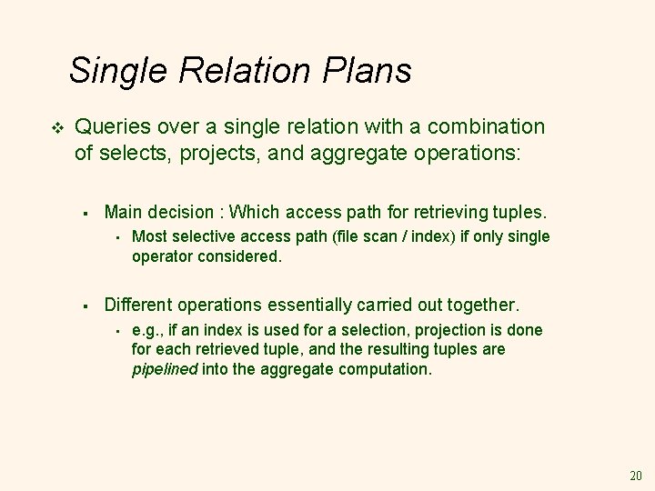
Single Relation Plans v Queries over a single relation with a combination of selects, projects, and aggregate operations: § Main decision : Which access path for retrieving tuples. • § Most selective access path (file scan / index) if only single operator considered. Different operations essentially carried out together. • e. g. , if an index is used for a selection, projection is done for each retrieved tuple, and the resulting tuples are pipelined into the aggregate computation. 20

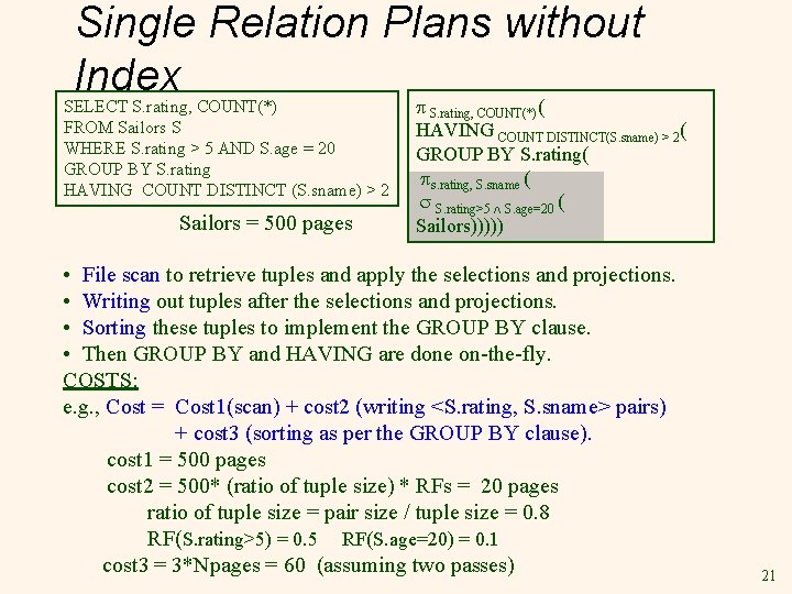
Single Relation Plans without Index SELECT S. rating, COUNT(*) FROM Sailors S WHERE S. rating > 5 AND S. age = 20 GROUP BY S. rating HAVING COUNT DISTINCT (S. sname) > 2 Sailors = 500 pages S. rating, COUNT(*)( HAVING COUNT DISTINCT(S. sname) > 2 ( GROUP BY S. rating( s. rating, S. sname ( S. rating>5 S. age=20 ( Sailors))))) • File scan to retrieve tuples and apply the selections and projections. • Writing out tuples after the selections and projections. • Sorting these tuples to implement the GROUP BY clause. • Then GROUP BY and HAVING are done on-the-fly. COSTS: e. g. , Cost = Cost 1(scan) + cost 2 (writing <S. rating, S. sname> pairs) + cost 3 (sorting as per the GROUP BY clause). cost 1 = 500 pages cost 2 = 500* (ratio of tuple size) * RFs = 20 pages ratio of tuple size = pair size / tuple size = 0. 8 RF(S. rating>5) = 0. 5 RF(S. age=20) = 0. 1 cost 3 = 3*Npages = 60 (assuming two passes) 21

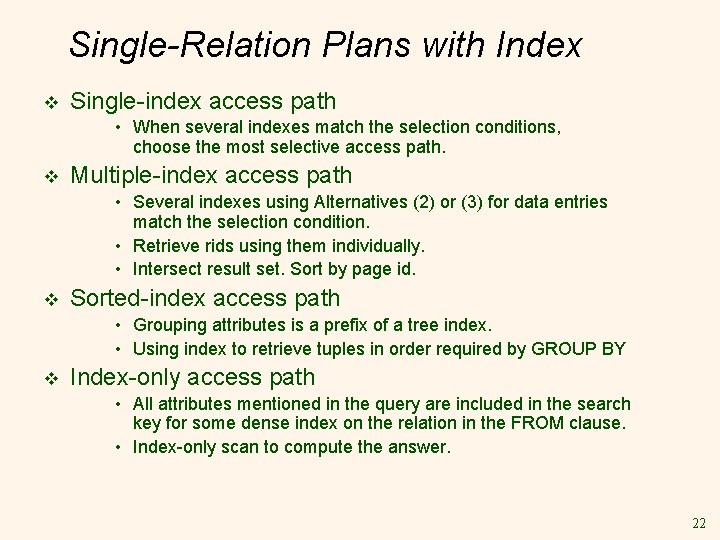
Single-Relation Plans with Index v Single-index access path • When several indexes match the selection conditions, choose the most selective access path. v Multiple-index access path • Several indexes using Alternatives (2) or (3) for data entries match the selection condition. • Retrieve rids using them individually. • Intersect result set. Sort by page id. v Sorted-index access path • Grouping attributes is a prefix of a tree index. • Using index to retrieve tuples in order required by GROUP BY v Index-only access path • All attributes mentioned in the query are included in the search key for some dense index on the relation in the FROM clause. • Index-only scan to compute the answer. 22

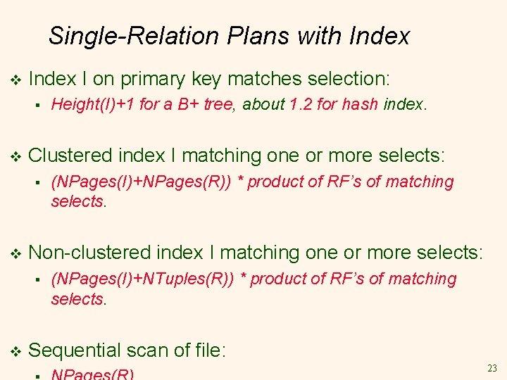
Single-Relation Plans with Index v Index I on primary key matches selection: § v Clustered index I matching one or more selects: § v (NPages(I)+NPages(R)) * product of RF’s of matching selects. Non-clustered index I matching one or more selects: § v Height(I)+1 for a B+ tree, about 1. 2 for hash index. (NPages(I)+NTuples(R)) * product of RF’s of matching selects. Sequential scan of file: 23

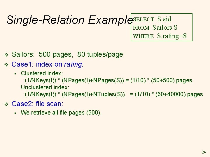
S. sid Single-Relation Example. SELECT FROM Sailors S WHERE v v Sailors: 500 pages, 80 tuples/page Case 1: index on rating. § v S. rating=8 Clustered index: (1/NKeys(I)) * (NPages(I)+NPages(S)) = (1/10) * (50+500) pages Unclustered index: (1/NKeys(I)) * (NPages(I)+NTuples(S)) = (1/10) * (50+40000) pages Case 2: file scan: § We retrieve all file pages (500). 24

Queries Over Multiple Relations § As the number of joins increases, the number of alternative plans grows rapidly § We need to restrict search space ! 25

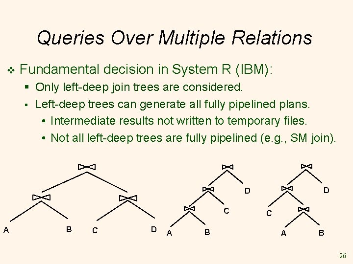
Queries Over Multiple Relations v Fundamental decision in System R (IBM): § Only left-deep join trees are considered. § Left-deep trees can generate all fully pipelined plans. • Intermediate results not written to temporary files. • Not all left-deep trees are fully pipelined (e. g. , SM join). D D C A B C D A B C A B 26

Enumeration of Left-Deep Plans v Left-deep plans differ in : § the order of relations, § the access method for each relation, and § the join method for each join. 27

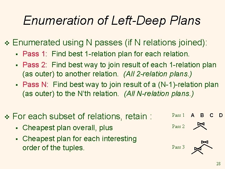
Enumeration of Left-Deep Plans v Enumerated using N passes (if N relations joined): § § § v Pass 1: Find best 1 -relation plan for each relation. Pass 2: Find best way to join result of each 1 -relation plan (as outer) to another relation. (All 2 -relation plans. ) Pass N: Find best way to join result of a (N-1)-relation plan (as outer) to the N’th relation. (All N-relation plans. ) For each subset of relations, retain : § § Cheapest plan overall, plus Cheapest plan for each interesting order of the tuples. Pass 1 A B C D Pass 2 Pass 3 28

Enumeration of Left-Deep Plans : Pass 1 v Identify selection terms in WHERE clause that mention only attributes of A: § perform access of A, before Join v Identify attributes of A not mentioned in SELECT or WHERE: § project out with first access of A, before Join v Keep cheapest overall plan for fetching all tuples : § a file scan v Keep cheapest plan with tuples in search key order : § B+ tree index 29

Left-Deep Plans: All 2 -relation Plans § Each single-relation plan from Pass 1 as outer relation, and every other relation as inner relation. § Examine WHERE clauses: • Selections involving only attributes of inner relation (apply before Join). • Selections defining the Join. • Selections involving attributes of other relations (apply after Join). § Only selections that are really applied before the join are those that match the chosen access paths for A and B. § Depending on the Join algorithm chosen, the cost may include materializing the outer relation. 30

Enumeration of Plans (Contd. ) v ORDER BY, GROUP BY, and aggregates handled as a final step, using either an `interestingly ordered’ plan or an additional sorting operator. v An N-1 way plan is not combined with another relation unless join condition between them : § v avoid Cartesian products if possible. Inspite of pruning plan space, this approach is still exponential in the # of tables. 31

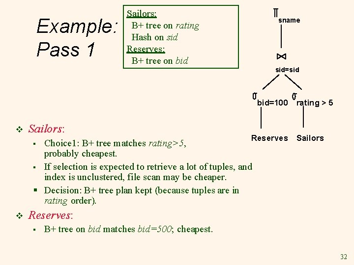
Example: Pass 1 Sailors: B+ tree on rating Hash on sid Reserves: B+ tree on bid sname sid=sid bid=100 rating > 5 v Sailors: Reserves Sailors Choice 1: B+ tree matches rating>5, probably cheapest. § If selection is expected to retrieve a lot of tuples, and index is unclustered, file scan may be cheaper. § Decision: B+ tree plan kept (because tuples are in rating order). § v Reserves: § B+ tree on bid matches bid=500; cheapest. 32

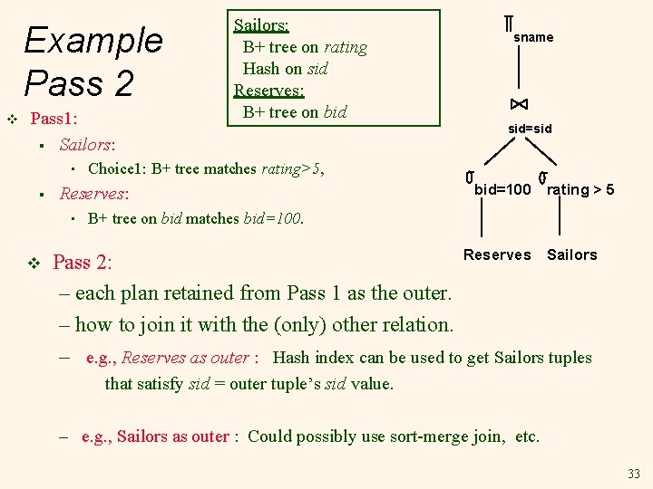
Example Pass 2 v Pass 1: § Sailors: • § sname sid=sid Choice 1: B+ tree matches rating>5, Reserves: • v Sailors: B+ tree on rating Hash on sid Reserves: B+ tree on bid=100 rating > 5 B+ tree on bid matches bid=100. Reserves Sailors Pass 2: – each plan retained from Pass 1 as the outer. – how to join it with the (only) other relation. – e. g. , Reserves as outer : Hash index can be used to get Sailors tuples that satisfy sid = outer tuple’s sid value. – e. g. , Sailors as outer : Could possibly use sort-merge join, etc. 33

Highlights of System R Optimizer v Impact of R Optimizer: § v Cost estimation: “Approximate art”. § § v Most widely used currently; works well for < 10 joins. Statistics, maintained in system catalog, used to estimate cost of operations and result sizes. Considers combination of CPU and I/O costs. Plan Space: Too large, must be pruned. § Only the space of left-deep plans considered. • Left-deep plans allow output of each operator to be pipelined into next operator without storing it in temporary relation. § Cartesian products avoided. 36

Other Approaches to Query Optimization v Exclusive search is not suitable for large number of Joins. v Rule-based optimizers: a set of rules to guide the generation of candidate plans. v Randomized plan generation: probabilistic algorithms to explore a large space of plans. v Estimating the size of intermediate relations accurately. • Parametric query optimization: find good plans for a given query for each of several different conditions that might be encountered at run-time. • Multiple-query optimization: take concurrent execution of several queries into account. 37

Summary : Query Optimization § Consider a set of alternative plans. • Must prune search space; • Typically, left-deep plans only; • Algorithms to explore alternate plans § Must estimate cost of each plan that is considered. • Estimate size of result of each operator • Estimate cost for each plan node. • Key issues: Statistics, indexes, operator implementations. 38