Relational Database Design Normalization 1 Informal Design Guidelines

Relational Database Design Normalization 1

Informal Design Guidelines for Relational Databases • What is relational database design? The grouping of attributes to form "good" relation schemas • What are the criteria for "good" base relations? – Semantics of the attributes – Problems with update anomalies – Null values in tuples – Spurious tuples 2

Criteria for “good” relations • GUIDELINE 1 (semantics of attributes): Informally, each tuple in a relation should represent one entity or relationship instance. (Applies to individual relations and their attributes). • Attributes of different entities (EMPLOYEEs, DEPARTMENTs, PROJECTs) should not be mixed in the same relation • Only foreign keys should be used to refer to other entities • Entity and relationship attributes should be kept apart as much as possible. • Mixing attributes of multiple entities may cause problems • Information when stored redundantly waste storage 3

EXAMPLE OF AN UPDATE ANOMALY Consider the relation: EMP_PROJ ( Emp#, Proj#, Ename, Pname, No_hours) • Update Anomaly: Changing the name of project number P 1 from “Billing” to “Customer-Accounting” may cause this update to be made for all 100 employees working on project P 1. • Insert Anomaly: Cannot insert a project unless an employee is assigned to. Inversely - Cannot insert an employee unless he/she is assigned to a project. • Delete Anomaly: When a project is deleted, it will result in deleting all the employees who work on that project. Alternately, if an employee is the sole employee on a project, deleting that employee would result in deleting the corresponding project. 4

Problems with update anomalies • GUIDELINE 2 (update anomalies): Design a schema that does not suffer from the insertion, deletion and update anomalies. If there any present, then note them so that applications can be made to take them into account • GUIDELINE 3 (Null values): Relations should be designed such that their tuples will have as few NULL values as possible • Attributes that are NULL frequently could be placed in separate relations (with the primary key) • Reasons for nulls: – attribute not applicable or invalid – attribute value unknown (may exist) – value known to exist, but unavailable 5

Spurious Tuples • • • Bad designs for a relational database may result in erroneous results for certain JOIN operations The "lossless join" property is used to guarantee meaningful results for join operations GUIDELINE 4: The relations should be designed to satisfy the lossless join condition. No spurious tuples should be generated by doing a natural -join of any relations. There are two important properties of decompositions: (a) non-additive or losslessness of the corresponding join (b) preservation of the functional dependencies. Note that property (a) is extremely important and cannot be sacrificed. Property (b) is less stringent and may be sacrificed. 6

Banking Schema branch (branch_name, branch_city, assets) customer (customer_name, customer_street, customer_city) account (account_number, branch_name, balance) loan (loan_number, branch_name, amount) depositor (customer_name, account_number) borrower (customer_name, loan_number) 7

Combine Schemas? • Suppose we combine borrower and loan to get bor_loan = (customer_id, loan_number, amount ) • Result is possible repetition of information (L-100 in example below) 8

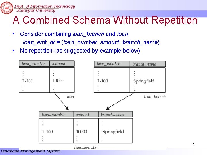
A Combined Schema Without Repetition • Consider combining loan_branch and loan_amt_br = (loan_number, amount, branch_name) • No repetition (as suggested by example below) 9

Overall Database Design Process • We have assumed schema R is given – R could have been generated when converting E-R diagram to a set of tables. – R could have been a single relation containing all attributes that are of interest (called universal relation). – Normalization breaks R into smaller relations. – R could have been the result of some ad hoc design of relations, which we then test/convert to normal form. 10

ER Model and Normalization • When an E-R diagram is carefully designed, identifying all entities correctly, the tables generated from the E-R diagram should not need further normalization. • However, in a real (imperfect) design, there can be functional dependencies from non-key attributes of an entity to other attributes of the entity – Example: an employee entity with attributes department_number and department_address, and a functional dependency department_number department_address – Good design would have made department an entity • Functional dependencies from non-key attributes of a relationship set possible, but rare --- most relationships are binary 11

What About Smaller Schemas? • Suppose we had started with bor_loan. How would we know to split up (decompose) it into borrower and loan? • In bor_loan, because loan_number is not a candidate key, the amount of a loan may have to be repeated. This indicates the need to decompose bor_loan. 12

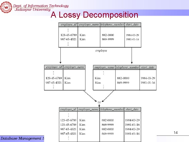
What About Smaller Schemas? • Not all decompositions are good. Suppose we decompose employee (employee_id, employee_name, telephone_number, start_date) into employee 1 = (employee_id, employee_name) employee 2 = (employee_name, telephone_number, start_date) • The next slide shows how we lose information -- we cannot reconstruct the original employee relation -- and so, this is a lossy decomposition. 13

A Lossy Decomposition 14

Relationships of Normal Forms 15

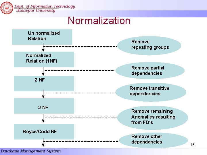
Normalization Un normalized Relation Remove repeating groups Normalized Relation (1 NF) Remove partial dependencies 2 NF Remove transitive dependencies 3 NF Boyce/Codd NF Remove remaining Anomalies resulting from FD‘s Remove other dependencies 16

First Normal Form • Domain is atomic if its elements are considered to be indivisible units – Examples of non-atomic domains: • Set of names, composite attributes • Identification numbers like CS 101 that can be broken up into parts • A relational schema R is in first normal form if the domains of all attributes of R are atomic • Non-atomic values: complicated storage and encourage redundant (repeated) storage of data • We assume all relations are in first normal form 17

First Normal Form (Cont’d) • Atomicity is actually a property of how the elements of the domain are used. – Example: Strings would normally be considered indivisible – Suppose that students are given roll numbers which are strings of the form CS 0012 or EE 1127 – If the first two characters are extracted to find the department, the domain of roll numbers is not atomic. 18

Functional Dependencies • Normalization theory is based on the concepts of normal forms. • A relational table is said to be a particular normal form if it satisfied a certain set of constraints. • FDs and keys are used to define normal forms for relations • A set of attributes X functionally determines a set of attributes Y if the value of X determine a unique value for Y • X -> Y holds if whenever two tuples have the same value for X, they must have the same value for Y • For any two tuples t 1 and t 2 in any relation instance r(R): If t 1[X]=t 2[X], then t 1[Y]=t 2[Y] • X -> Y in R specifies a constraint on all relation instances r(R) • FDs are derived from the real-world constraints on the attributes 19

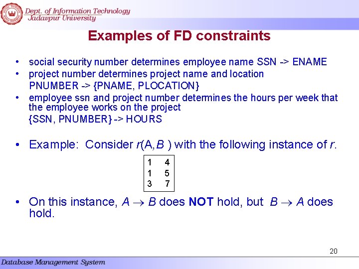
Examples of FD constraints • social security number determines employee name SSN -> ENAME • project number determines project name and location PNUMBER -> {PNAME, PLOCATION} • employee ssn and project number determines the hours per week that the employee works on the project {SSN, PNUMBER} -> HOURS • Example: Consider r(A, B ) with the following instance of r. 1 1 3 4 5 7 • On this instance, A B does NOT hold, but B A does hold. 20

Examples of FD constraints • An FD is a property of the attributes in the schema R • The constraint must hold on every relation instance r(R) • If K is a key of R, then K functionally determines all attributes in R (since we never have two distinct tuples with t 1[K]=t 2[K]) • K is a superkey for relation schema R if and only if K R • K is a candidate key for R if and only if – K R, and – for no K, R • Consider the schema: bor_loan = (customer_id, loan_number, amount ). We expect this functional dependency to hold: loan_number amount but would not expect the following to hold: amount customer_name 21

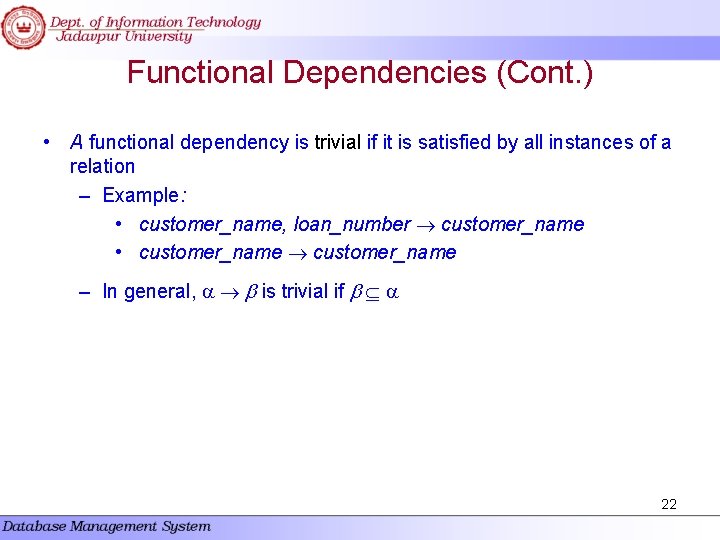
Functional Dependencies (Cont. ) • A functional dependency is trivial if it is satisfied by all instances of a relation – Example: • customer_name, loan_number customer_name • customer_name – In general, is trivial if 22

Inference Rules for FDs • Given a set of FDs F, we can infer additional FDs that hold whenever the FDs in F hold Armstrong's inference rules: IR 1. (Reflexive) If Y subset-of X, then X -> Y IR 2. (Augmentation) If X -> Y, then XZ -> YZ (Notation: XZ stands for X U Z) IR 3. (Transitive) If X -> Y and Y -> Z, then X -> Z • These rules are – sound (generate only functional dependencies that actually hold) and – complete (generate all functional dependencies that hold). 23

Inference Rules for FDs Some additional inference rules that are useful: (Decomposition) If X -> YZ, then X -> Y and X -> Z (Union) If X -> Y and X -> Z, then X -> YZ (Psuedotransitivity) If X -> Y and WY -> Z, then WX -> Z • The last three inference rules, as well as any other inference rules, can be deduced from IR 1, IR 2, and IR 3 (completeness property) 24

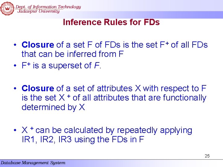
Inference Rules for FDs • Closure of a set F of FDs is the set F+ of all FDs that can be inferred from F • F+ is a superset of F. • Closure of a set of attributes X with respect to F is the set X + of all attributes that are functionally determined by X • X + can be calculated by repeatedly applying IR 1, IR 2, IR 3 using the FDs in F 25

Example of F+ • R = (A, B, C, G, H, I) F={ A B A C CG H CG I B H} • some members of F+ – A H • by transitivity from A B and B H – AG I • by augmenting A C with G, to get AG CG and then transitivity with CG I – CG HI • by augmenting CG I to infer CG CGI, and augmenting of CG H to infer CGI HI, and then transitivity 26

Procedure for Computing F+ • To compute the closure of a set of functional dependencies F: F+=F repeat for each functional dependency f in F+ apply reflexivity and augmentation rules on f add the resulting functional dependencies to F + for each pair of functional dependencies f 1 and f 2 in F + if f 1 and f 2 can be combined using transitivity then add the resulting functional dependency to F + until F + does not change any further NOTE: We shall see an alternative procedure for this task later 27

Closure of Functional Dependencies (Cont. ) • We can further simplify manual computation of F+ by using the following additional rules. – If holds and holds, then holds (union) – If holds, then holds and holds (decomposition) – If holds and holds, then holds (pseudotransitivity) 28

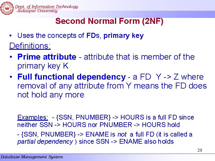
Second Normal Form (2 NF) • Uses the concepts of FDs, primary key Definitions: • Prime attribute - attribute that is member of the primary key K • Full functional dependency - a FD Y -> Z where removal of any attribute from Y means the FD does not hold any more Examples: - {SSN, PNUMBER} -> HOURS is a full FD since neither SSN -> HOURS nor PNUMBER -> HOURS hold - {SSN, PNUMBER} -> ENAME is not a full FD (it is called a partial dependency ) since SSN -> ENAME also holds 29

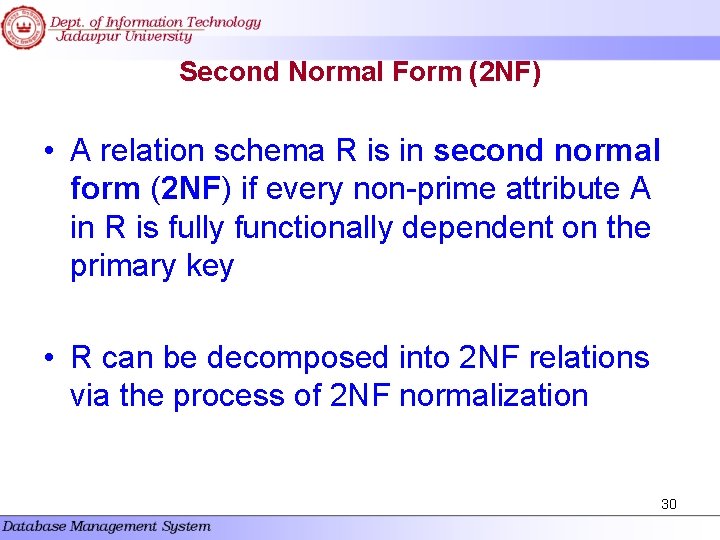
Second Normal Form (2 NF) • A relation schema R is in second normal form (2 NF) if every non-prime attribute A in R is fully functionally dependent on the primary key • R can be decomposed into 2 NF relations via the process of 2 NF normalization 30

Normalization An Example : A company obtains parts from a number of suppliers. Each supplier is located in one city. A city can have more than one supplier located there and each city has a status code associated with it. Each supplier may provide many parts. The company creates a simple relational table to store this information: FIRST (s#, status, city, p#, qty) s# status City p# Qty Supplier identification number Status code assigned to city City where supplier is located Part number of part supplied Qty of parts supplied to date Composite primary key is (s#, p#) 31

Normalization • FIRST NORMAL FORM – 1 NF s# city s 1 s 1 s 2 s 3 London Paris Tokyo status p# 20 20 10 10 30 30 p 1 p 2 p 3 p 4 p 1 p 3 p 2 p 4 qty 300 100 250 100 300 200 32

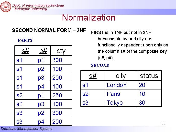
Normalization SECOND NORMAL FORM – 2 NF PARTS s# s 1 s 1 s 2 s 3 p# p 1 p 2 p 3 p 4 p 1 p 3 p 2 p 4 qty 300 100 250 100 300 200 FIRST is in 1 NF but not in 2 NF because status and city are functionally dependent upon only on the column s# of the composite key (s#, p#). SECOND s# s 1 s 2 s 3 city London Paris Tokyo status 20 10 30 33

Goals of Normalization • Let R be a relation scheme with a set F of functional dependencies. • Decide whether a relation scheme R is in “good” form. • In the case that a relation scheme R is not in “good” form, decompose it into a set of relation scheme {R 1, R 2, . . . , Rn} such that – each relation scheme is in good form – the decomposition is a lossless-join decomposition – Preferably, the decomposition should be dependency preserving. 34

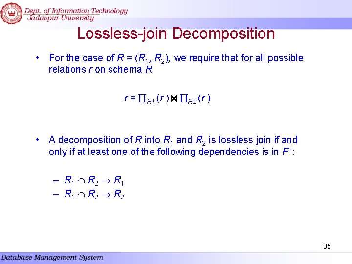
Lossless-join Decomposition • For the case of R = (R 1, R 2), we require that for all possible relations r on schema R r = R 1 (r ) R 2 (r ) • A decomposition of R into R 1 and R 2 is lossless join if and only if at least one of the following dependencies is in F+: – R 1 R 2 R 1 – R 1 R 2 35

Example of Relation Decomposition 36

Dependency Preservation Decomposition • Definition: Each FD specified in F either appears directly in one of the relations in the decomposition, or be inferred from FDs that appear in some relation. 37

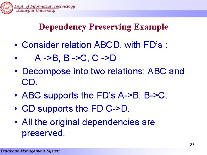
Dependency Preserving Example • Consider relation ABCD, with FD’s : • A ->B, B ->C, C ->D • Decompose into two relations: ABC and CD. • ABC supports the FD’s A->B, B->C. • CD supports the FD C->D. • All the original dependencies are preserved. 38

Boyce-Codd Normal Form A relation schema R is in BCNF with respect to a set F of functional dependencies if for all functional dependencies in F+ of the form where R and R, at least one of the following holds: • is trivial (i. e. , ) • is a superkey for R Example schema not in BCNF: bor_loan = ( customer_id, loan_number, amount ) because loan_number amount holds on bor_loan but loan_number is not a superkey 39

Decomposing a Schema into BCNF • Suppose we have a schema R and a non-trivial dependency causes a violation of BCNF. We decompose R into: ( U ) (R-( - )) • In our example, – = loan_number – = amount and bor_loan is replaced by – ( U ) = ( loan_number, amount ) – ( R - ( - ) ) = ( customer_id, loan_number ) • • 40

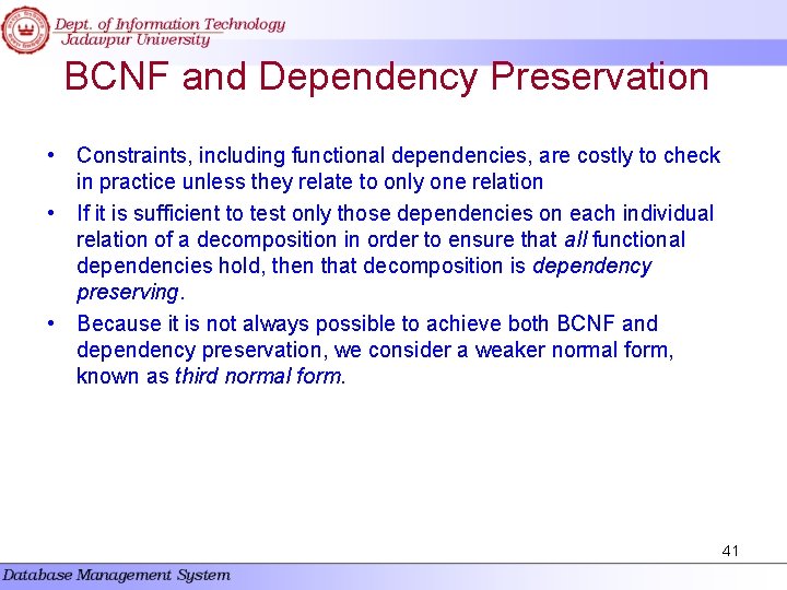
BCNF and Dependency Preservation • Constraints, including functional dependencies, are costly to check in practice unless they relate to only one relation • If it is sufficient to test only those dependencies on each individual relation of a decomposition in order to ensure that all functional dependencies hold, then that decomposition is dependency preserving. • Because it is not always possible to achieve both BCNF and dependency preservation, we consider a weaker normal form, known as third normal form. 41

Third Normal Form: Motivation • There are some situations where – BCNF is not dependency preserving, and – efficient checking for FD violation on updates is important • Solution: define a weaker normal form, called Third Normal Form (3 NF) – Allows some redundancy (with resultant problems; we will see examples later) – But functional dependencies can be checked on individual relations without computing a join. – There is always a lossless-join, dependency-preserving decomposition into 3 NF. 42

Third Normal Form • A relation schema R is in third normal form (3 NF) if for all: in F+ at least one of the following holds: – is trivial (i. e. , ) – is a superkey for R – Each attribute A in – is contained in a candidate key for R. (NOTE: each attribute may be in a different candidate key) • If a relation is in BCNF it is in 3 NF (since in BCNF one of the first two conditions above must hold). • Third condition is a minimal relaxation of BCNF to ensure dependency preservation (will see why later). 43

Normalization • THIRD NORMAL FORM – 3 NF A relational table is in third normal form (3 NF) if it is already in 2 NF and every non-key column is non transitively dependent upon its primary key. In other words, all non-key attributes are functionally dependent only upon the primary key. SUPPLIER s# city s 1 s 2 s 3 s 4 London Paris Tokyo Paris status 20 10 30 10 The table supplier is in 2 NF but not in 3 NF because it contains a transitive dependency SUPPLIER. s# —> SUPPLIER. city —> SUPPLIER. status SUPPLIER. s# —> SUPPLIER. status 44

Normalization CITY_STATUS SUPPLIER s# The transformation of SUPPLIER into 3 NF s 1 s 2 s 3 s 4 s 5 city London Paris Tokyo Paris London city London Paris Tokyo Rome status 20 10 30 50 45

Comparison of BCNF and 3 NF • It is always possible to decompose a relation into a set of relations that are in 3 NF such that: – the decomposition is lossless – the dependencies are preserved • It is always possible to decompose a relation into a set of relations that are in BCNF such that: – the decomposition is lossless – it may not be possible to preserve dependencies. 46

BCNF and Dependency Preservation • Constraints, including functional dependencies, are costly to check in practice unless they relate to only one relation • If it is sufficient to test only those dependencies on each individual relation of a decomposition in order to ensure that all functional dependencies hold, then that decomposition is dependency preserving. • Because it is not always possible to achieve both BCNF and dependency preservation, we consider a weaker normal form, known as third normal form. 47

How good is BCNF? • There are database schemas in BCNF that do not seem to be sufficiently normalized • Consider a database classes (course, teacher, book ) such that (c, t, b) classes means that t is qualified to teach c, and b is a required textbook for c • The database is supposed to list for each course the set of teachers any one of which can be the course’s instructor, and the set of books, all of which are required for the course (no matter who teaches it). 48

How good is BCNF? (Cont. ) course database database operating systems teacher Avi Hank Sudarshan Avi Pete book DB Concepts Ullman OS Concepts Stallings classes • There are no non-trivial functional dependencies and therefore the relation is in BCNF • Insertion anomalies – i. e. , if Marilyn is a new teacher that can teach database, two tuples need to be inserted (database, Marilyn, DB Concepts) (database, Marilyn, Ullman) 49

How good is BCNF? (Cont. ) • Therefore, it is better to decompose classes into: course teacher database operating systems Avi Hank Sudarshan Avi Jim teaches course book database operating systems DB Concepts Ullman OS Concepts Shaw text This suggests the need for higher normal forms, such as Fourth Normal Form (4 NF), which we shall see later. 50

Fourth Normal Form • A relation schema R is in 4 NF if and only if, whenever there exist subsets A and B of the attributes of R such that the MVD A B is satisfied then all attributes of R are also functionally dependent on A. • If a relation is in 4 NF it is in BCNF and all MVDs in R are in fact FDs out of the candidate key. 51

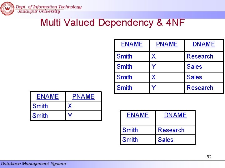
Multi Valued Dependency & 4 NF ENAME PNAME DNAME Smith X Research Smith Y Sales Smith X Sales Smith Y Research PNAME Smith X Smith Y ENAME DNAME Smith Research Smith Sales 52

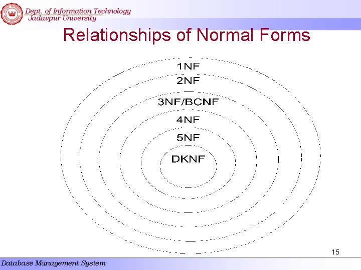
Further Normal Forms The advanced forms of normalization are: Ø Fourth Normal Form (4 NF) Ø Fifth Normal Form (5 NF or PJNF) Ø Domain-key Normal Form (DKNF) • Join dependencies generalize multivalued dependencies – lead to project-join normal form (PJ/NF) (also called fifth normal form) • A class of even more general constraints, leads to a normal form called domain-key normal form. • Problem with these generalized constraints: are hard to reason with, and no set of sound and complete set of inference rules exists. • Hence rarely used 53

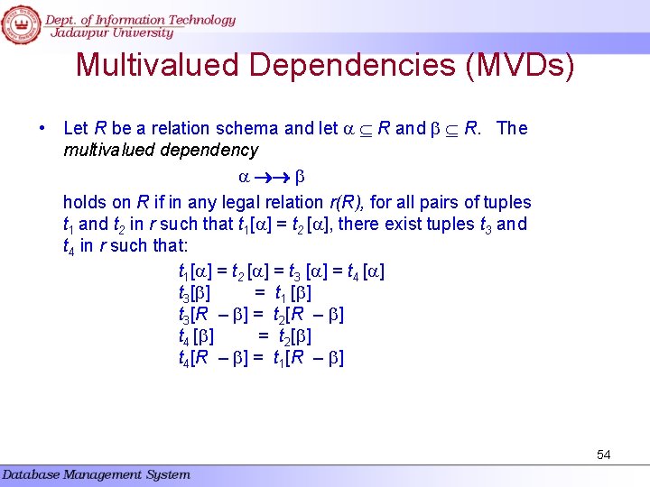
Multivalued Dependencies (MVDs) • Let R be a relation schema and let R and R. The multivalued dependency holds on R if in any legal relation r(R), for all pairs of tuples t 1 and t 2 in r such that t 1[ ] = t 2 [ ], there exist tuples t 3 and t 4 in r such that: t 1[ ] = t 2 [ ] = t 3 [ ] = t 4 [ ] t 3[ ] = t 1 [ ] t 3[R – ] = t 2[R – ] t 4 [ ] = t 2[ ] t 4[R – ] = t 1[R – ] 54

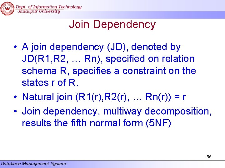
Join Dependency • A join dependency (JD), denoted by JD(R 1, R 2, … Rn), specified on relation schema R, specifies a constraint on the states r of R. • Natural join (R 1(r), R 2(r), … Rn(r)) = r • Join dependency, multiway decomposition, results the fifth normal form (5 NF) 55

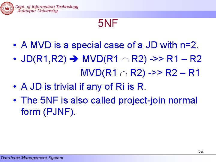
5 NF • A MVD is a special case of a JD with n=2. • JD(R 1, R 2) MVD(R 1 R 2) ->> R 1 – R 2 MVD(R 1 R 2) ->> R 2 – R 1 • A JD is trivial if any of Ri is R. • The 5 NF is also called project-join normal form (PJNF). 56

Join Dependency & 5 NF: A relation schema is in 5 NF or project-join normal form(PJNF) w. r. t a set of F of functional, multivalued and join dependencies if, for every join dependency JD(R 1, R 2, … , Rn) in closure of F, every Ri is a super key of R. 57

Join Dependency & 5 NF SNAME PARTNAME PROJNAME Smith Bolt Proj. X Smith Nut Proj. Y Brown Bolt Proj. Y John Nut Proj. Z Brown Nail Proj. X There is no MVD 4 NF; JD ( {SNAME PARTNAME} {PARTNAME PROJNAME} {SNAME PROJNAME} ) is not lossless no 5 NF 58

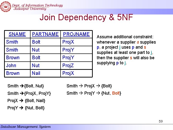
Join Dependency & 5 NF SNAME PARTNAME PROJNAME Smith Bolt Proj. X Smith Nut Proj. Y Brown Bolt Proj. Y John Nut Proj. Z Brown Nail Proj. X Assume additional constraint: whenever a supplier s supplies p, a project j uses p and s supplies at least one part to j, then the supplier s will also be supplying p to j. Smith {Bolt, Nut} Smith Proj. X {Bolt} Smith {Proj. X, Proj. Y} Smith Proj. Y {Nut, Bolt} Proj. X {Bolt, Nail} Proj. Y {Nut, Bolt} 59

Join Dependency & 5 NF SNAME PARTNAME PROJNAME Smith Bolt Proj. X Smith Nut Proj. Y Brown Bolt Proj. Y John Nut Proj. Z Brown Nail Proj. X Smith Brown Bolt Proj. Y Proj. X JD ( R 1 = {SNAME PARTNAME} R 2 = {PARTNAME PROJNAME} R 3 = {SNAME PROJNAME} ) is valid each in 5 NF 60

Inclusion Dependencies • To define certain inter-relation constraints. – FK (referential integrity) cannot be specified as the functional or multivalued dependency – The inclusion dependency R. X < S. Y between • The set of attributes X of R and the set of attributes Y of S • Specifies that at any specific time X(r(R)) Y(s(S)) • Must have same number of attributes. • Domain for each pair of corresponding attributes should be compatible. 61

Example • Department. dmgrssn <Employee. ssn • Employee. dnumber < department. dnumber • All the above represents the referential integrity constraints. • Employee. ssn < Person. ssn [specialization] 62

Domain-Key Normal Form (DKNF) • DKNF (the ultimate normal form, theoretically) • A relation R is said to be in DKNF if all constraints and dependencies that should hold on the relation can be enforced simple by enforcing the domain constraints and key constraints on the relation. • E. g. , car(name, vn#), manufacture(vn#, country) • If car id Toyota or Lexus and the manufacturer country is Japan, then first character is “J”, etc… • Value…, …. 63