Reintroduction to Open Mx Sarah Medland Starting at

(Re)introduction to Open. Mx Sarah Medland

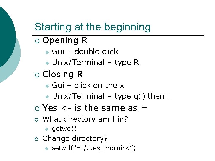
Starting at the beginning ¡ Opening R l l ¡ Gui – double click Unix/Terminal – type R Closing R l l Gui – click on the x Unix/Terminal – type q() then n ¡ Yes <- is the same as = ¡ What directory am I in? l ¡ getwd() Change directory? l setwd("H: /tues_morning”)

Starting at the beginning ¡ Data preparation l l l The algebra style used in Mx expects 1 line per case/family (Almost) limitless number of families and variables Data needs to be read into R before it can be analysed (the commands to read the data can be nested within the R script) ¡ Default missing code is now NA ¡

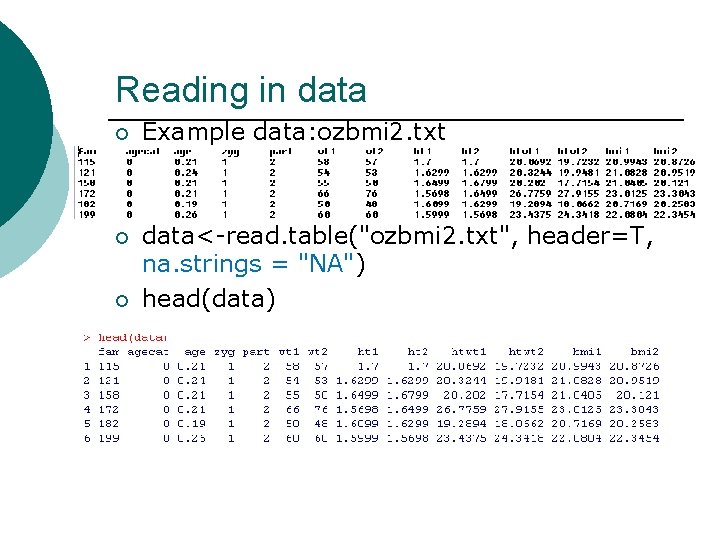
Reading in data ¡ Example data: ozbmi 2. txt ¡ data<-read. table("ozbmi 2. txt", header=T, na. strings = "NA") head(data) ¡

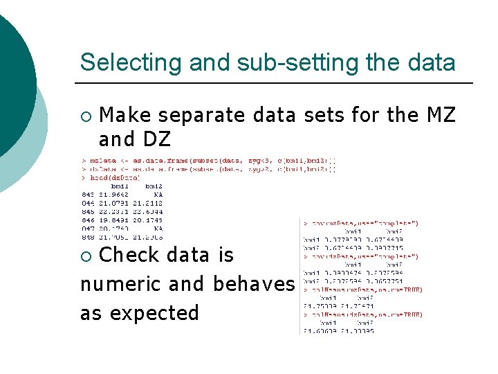
Selecting and sub-setting the data ¡ Make separate data sets for the MZ and DZ Check data is numeric and behaves as expected ¡

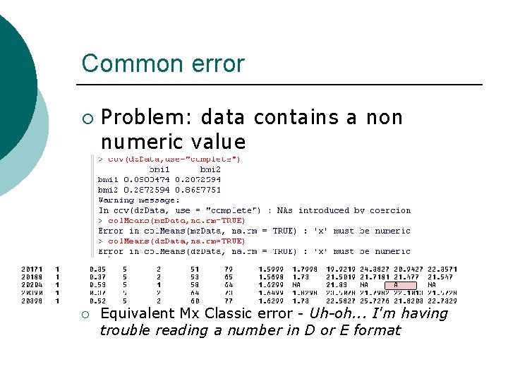
Common error ¡ ¡ Problem: data contains a non numeric value Equivalent Mx Classic error - Uh-oh. . . I'm having trouble reading a number in D or E format

Important structural stuff ¡ Mx Classic l Each job was composed of one or more groups Each group is ‘opened’ with a title ¡ Each group is ‘closed’ with an end statement ¡ ¡ open. Mx l Less structured

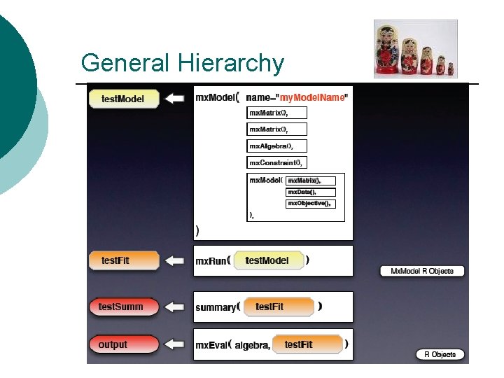
General Hierarchy

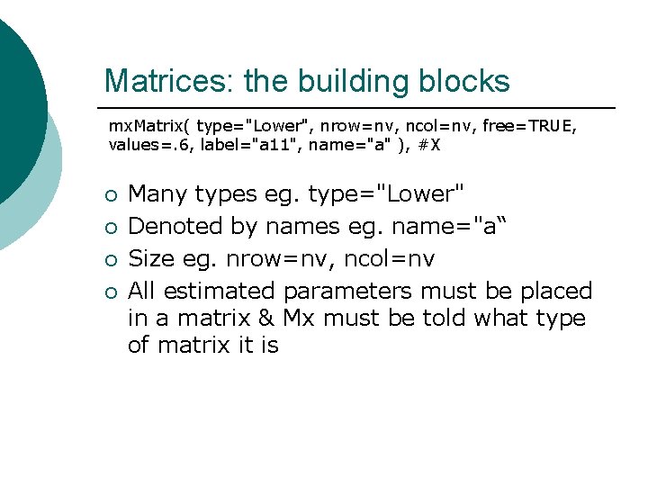
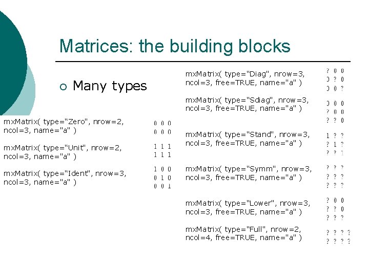
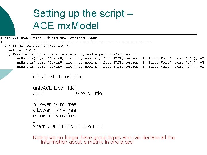
Matrices: the building blocks mx. Matrix( type="Lower", nrow=nv, ncol=nv, free=TRUE, values=. 6, label="a 11", name="a" ), #X ¡ ¡ Many types eg. type="Lower" Denoted by names eg. name="a“ Size eg. nrow=nv, ncol=nv All estimated parameters must be placed in a matrix & Mx must be told what type of matrix it is

Matrices: the building blocks ¡ Many types mx. Matrix( type=“Diag", nrow=3, ncol=3, free=TRUE, name="a" ) mx. Matrix( type=“Sdiag", nrow=3, ncol=3, free=TRUE, name="a" ) mx. Matrix( type=“Zero", nrow=2, ncol=3, name="a" ) mx. Matrix( type=“Unit", nrow=2, ncol=3, name="a" ) mx. Matrix( type=“Ident", nrow=3, ncol=3, name="a" ) mx. Matrix( type=“Stand", nrow=3, ncol=3, free=TRUE, name="a" ) mx. Matrix( type=“Symm", nrow=3, ncol=3, free=TRUE, name="a" ) mx. Matrix( type=“Lower", nrow=3, ncol=3, free=TRUE, name="a" ) mx. Matrix( type=“Full", nrow=2, ncol=4, free=TRUE, name="a" )

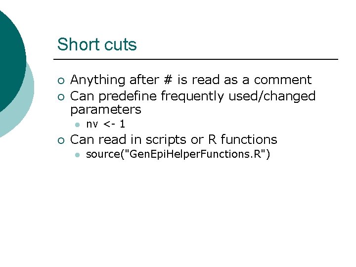
Short cuts ¡ ¡ Anything after # is read as a comment Can predefine frequently used/changed parameters l ¡ nv <- 1 Can read in scripts or R functions l source("Gen. Epi. Helper. Functions. R")

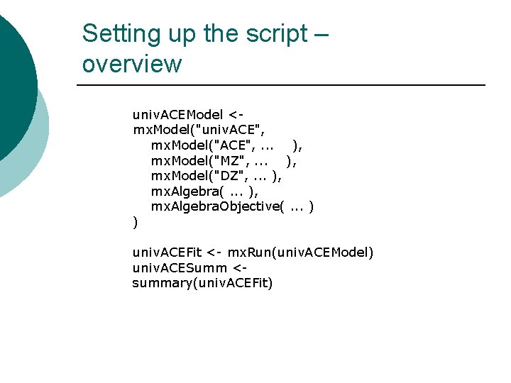
Setting up the script – overview univ. ACEModel <mx. Model("univ. ACE", mx. Model("ACE", . . . ), mx. Model("MZ", . . . ), mx. Model("DZ", . . . ), mx. Algebra(. . . ), mx. Algebra. Objective(. . . ) ) univ. ACEFit <- mx. Run(univ. ACEModel) univ. ACESumm <summary(univ. ACEFit)

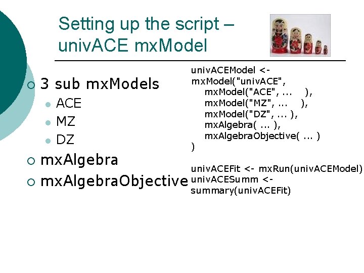
Setting up the script – univ. ACE mx. Model ¡ 3 sub mx. Models l l l ACE MZ DZ univ. ACEModel <mx. Model("univ. ACE", mx. Model("ACE", . . . ), mx. Model("MZ", . . . ), mx. Model("DZ", . . . ), mx. Algebra(. . . ), mx. Algebra. Objective(. . . ) ) mx. Algebra univ. ACEFit <- mx. Run(univ. ACEModel) ¡ mx. Algebra. Objective univ. ACESumm <¡ summary(univ. ACEFit)

Setting up the script – ACE mx. Model Classic Mx translation univ. ACE !Job Title ACE !Group Title … a Lower nv nv free c Lower nv nv free e Lower nv nv free … Start. 6 a 1 1 1 c 1 1 1 e 1 1 1 Notice we no longer have group types and can declare all the information about a matrix in one place!

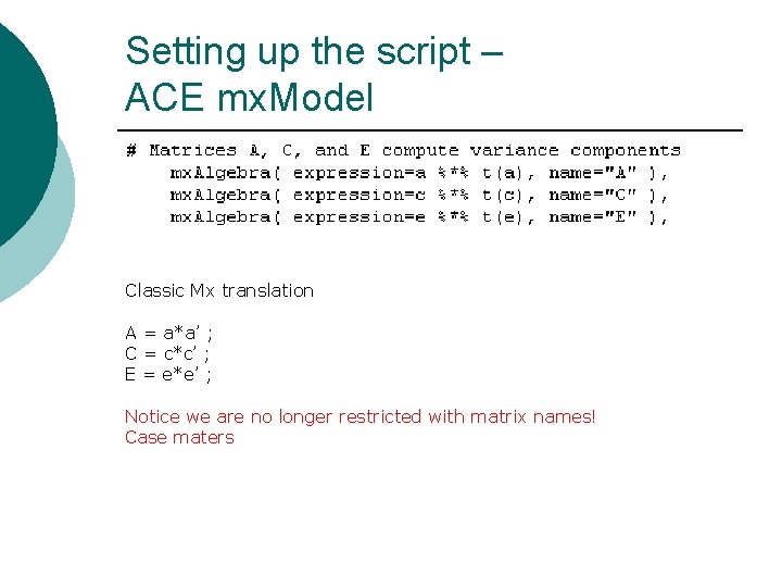
Setting up the script – ACE mx. Model Classic Mx translation A = a*a’ ; C = c*c’ ; E = e*e’ ; Notice we are no longer restricted with matrix names! Case maters

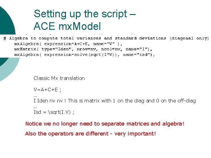
Setting up the script – ACE mx. Model Classic Mx translation V=A+C+E ; … I Iden nv nv ! This is matrix with 1 on the diag and 0 on the off-diag … Isd = sqrt(I. V) ; Notice we no longer need to separate matrices and algebra! Also the operators are different - very important!

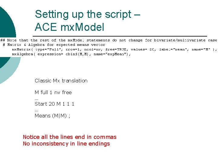
Setting up the script – ACE mx. Model Classic Mx translation M full 1 nv free … Start 20 M 1 1 1 … Means (M|M) ; Notice all the lines end in commas No inconsistency in line endings

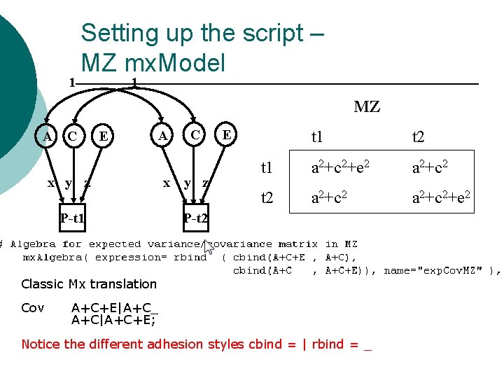
1 Setting up the script – MZ mx. Model 1 MZ A C E A x y z P-t 1 x C y z E t 1 t 2 t 1 a 2+c 2+e 2 a 2+c 2 t 2 a 2+c 2+e 2 P-t 2 Classic Mx translation Cov A+C+E|A+C_ A+C|A+C+E; Notice the different adhesion styles cbind = | rbind = _

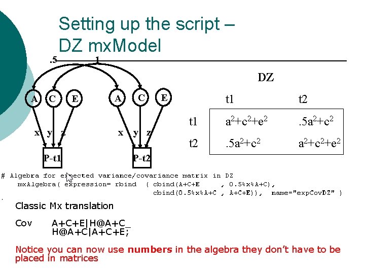
. 5 Setting up the script – DZ mx. Model 1 DZ A C E x y z A x P-t 1 C y z E t 1 t 2 t 1 a 2+c 2+e 2 . 5 a 2+c 2 t 2 . 5 a 2+c 2+e 2 P-t 2 Classic Mx translation Cov A+C+E|H@A+C_ H@A+C|A+C+E; Notice you can now use numbers in the algebra they don’t have to be placed in matrices

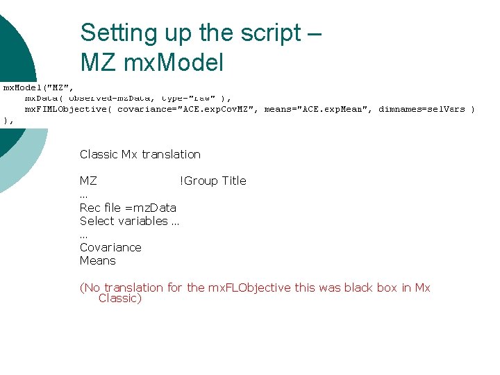
Setting up the script – MZ mx. Model Classic Mx translation MZ !Group Title … Rec file =mz. Data Select variables … … Covariance Means (No translation for the mx. FLObjective this was black box in Mx Classic)

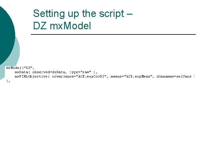
Setting up the script – DZ mx. Model

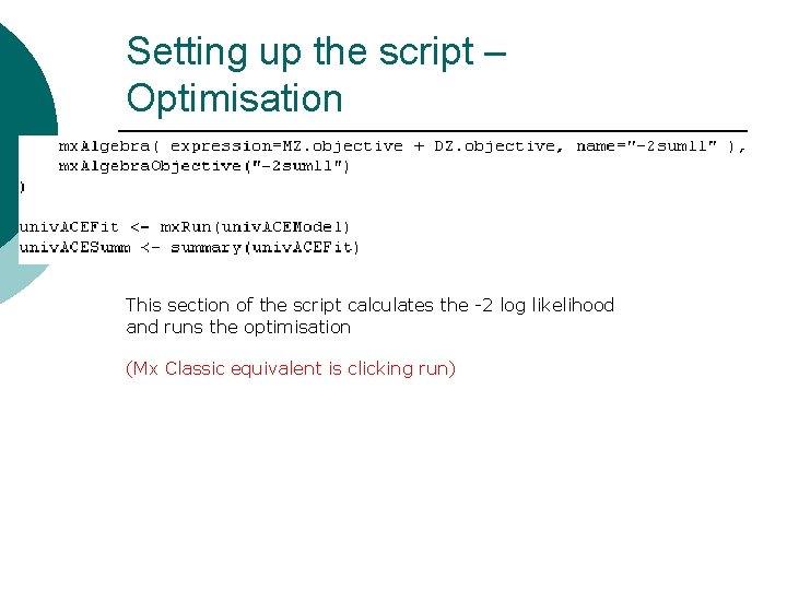
Setting up the script – Optimisation Classic Mx translation This section of the script calculates the -2 log likelihood and runs the optimisation (Mx Classic equivalent is clicking run)

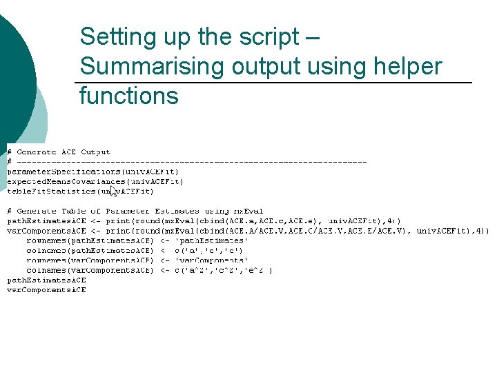
Setting up the script – Summarising output using helper functions

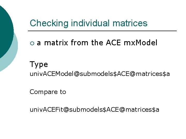
Checking individual matrices ¡ a matrix from the ACE mx. Model Type univ. ACEModel@submodels$ACE@matrices$a Compare to univ. ACEFit@submodels$ACE@matrices$a

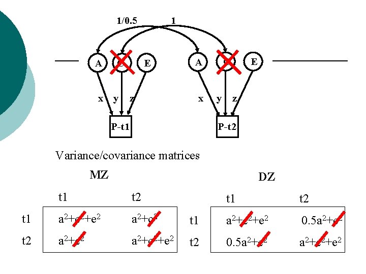
Testing for significance Set (one or more) estimated parameters to zero ¡ Known as ‘dropping’ the parameter from the model ¡ l ie dropping C

1/0. 5 A x C y 1 E z C A x P-t 1 y E z P-t 2 Variance/covariance matrices MZ DZ t 1 t 2 t 1 a 2+c 2+e 2 a 2+c 2 t 2 a 2+c 2+e 2 t 1 t 2 t 1 a 2+c 2+e 2 0. 5 a 2+c 2 t 2 0. 5 a 2+c 2+e 2

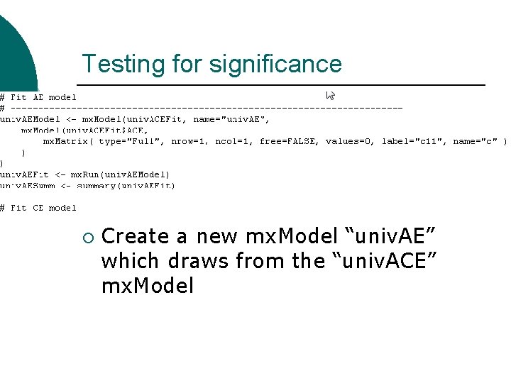
Testing for significance ¡ Create a new mx. Model “univ. AE” which draws from the “univ. ACE” mx. Model

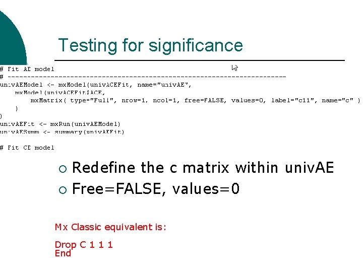
Testing for significance Redefine the c matrix within univ. AE ¡ Free=FALSE, values=0 ¡ Mx Classic equivalent is: Drop C 1 1 1 End

Saving your output ¡ Save the R workspace l l l ¡ On closing click yes Very big Saves everything Save the fitted model l Equivalent to save in classic Mx save(univ. ACEFit, file="test. omxs") load("test. omxs") – need to load Open. Mx first

What to report ¡ Summary statistics l ¡ Usually from a simplified ‘saturated’ model Standardized estimates l Easier to conceptualise ie 40% of the phenotypic variance vs a genetic effect of 2. 84 ¡ Can easily be returned to original scale if summary statistics are provided ¡

What to report ¡ Path coefficients l Very important in multivariate analyses ¡ Gives a much clearer picture of the directionality of effects Variance components/proportion of variance explained ¡ Genetic correlations ¡

General Advice/Problem solving Scripting styles differ ¡ Check the sample description ¡ Learn to love the webpage ¡ Comments are your friends ¡

Time for coffee explodingdog. com