Reinforcement Learning Tutorial Rethinking State Action Reward Satinder

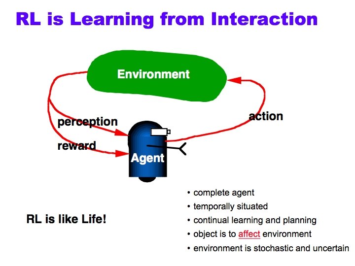
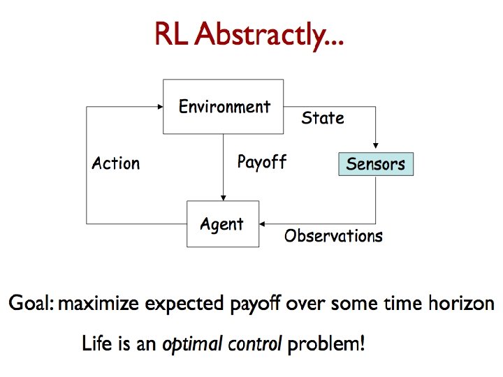
Reinforcement Learning: Tutorial + Rethinking State, Action & Reward Satinder Singh Computer Science & Engineering University of Michigan

Rich Sutton & Doina Precup Michael Littman Richard Lewis Andrew Barto Michael Kearns Matthew Rudary Erik Talvitie Britton Wolfe David Wingate Michael James Jonathan Sorg

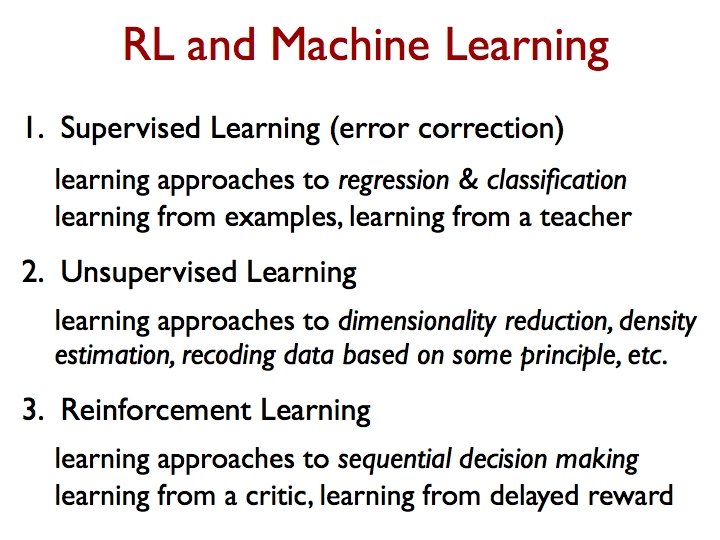
Outline • RL Tutorial – Markov Decision Processes (MDPs) – Policy Evaluation – Optimal Control • • Options (Rethinking Actions) Predictions (Rethinking States) Internal Rewards (Rethinking Rewards) Random Thought(s)

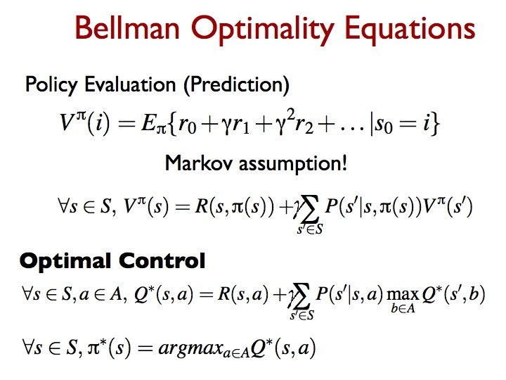
Markov Decision Process (MDP) • • • S: finite state space A: finite action space P: transition probabilities P(i|j, a) R: payoff function R(i) : deterministic policy V (i): return for policy when started in state i V (i) = E {r 0+ r 1 + 2 r 2 + 3 r 3+… | s 0=i} • *: optimal policy is argmax V

Planning (Policy Evaluation)

Planning (Optimal Control)

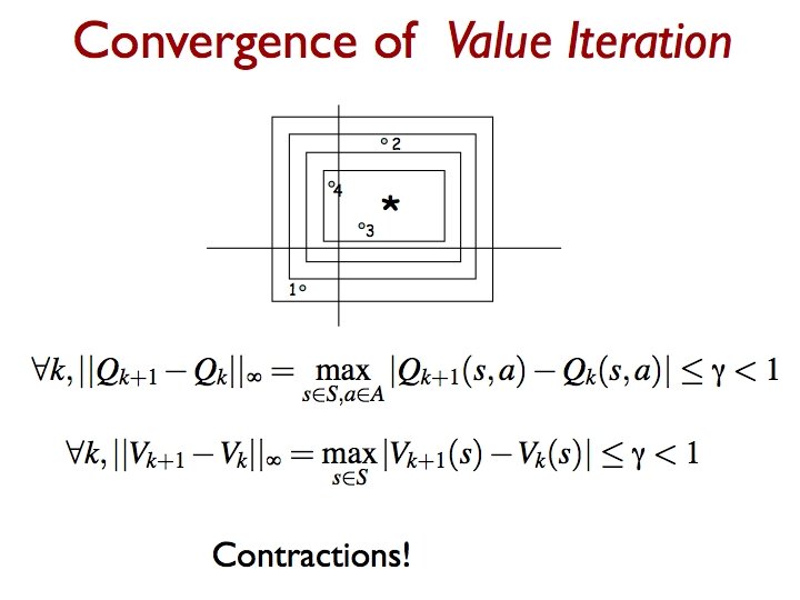
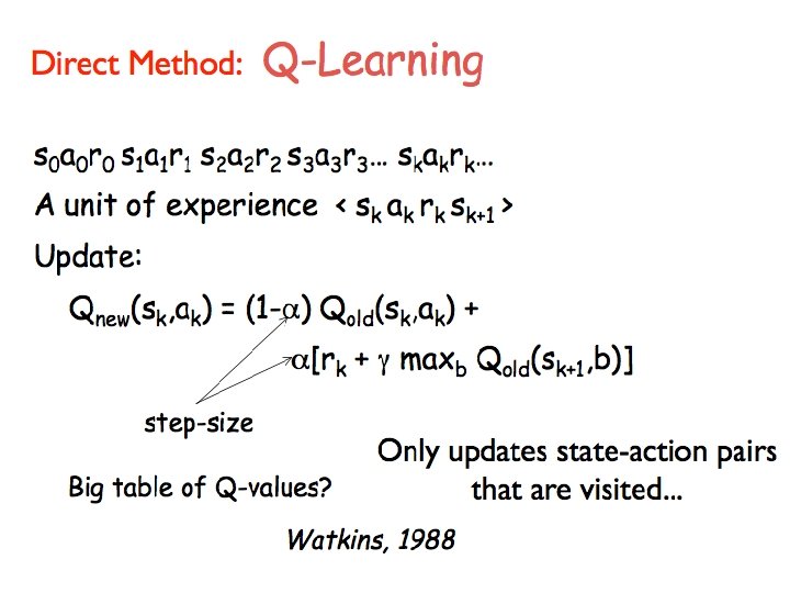
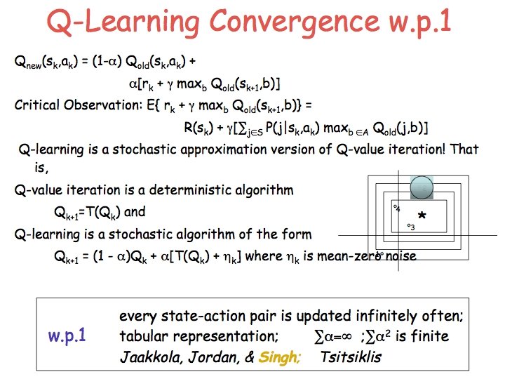
So far… • MDP definition • Policy Evaluation Problem – Planning (Iteration) – Learning (TD) • Optimal Control Problem – Planning (Q-value Iteration; Linear Programming) – Learning (Q-learning) Q-learning first provably convergent adaptive optimal control algorithm (Chris Watkins!) So why aren’t we done?

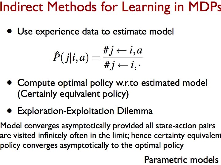
Exploration-Exploitation • Epsilon-Greedy – With small probability explore, else exploit – Suitably decreasing epsilon guarantees asymptotic convergence (GLIE: Singh, Jaakkola, Szepesvari & Littman) • Optimism Under Uncertainty – For arbitrary MDPs, guarantee convergence to near-optimal policy in sample and time complexity polynomial in reasonable size-parameters of the MDP (PAC style) • E 3 (Kearns & Singh), Rmax (Brafman & Tennenholtz), Metric-E 3 (Kakade, Kearns & Langford), MBIE (Strehl, Littman), others • Bayesian Methods – State space is state of knowledge (posteriors). In principle MDP methods including above extend (BAMDPs). So what is holding us back?

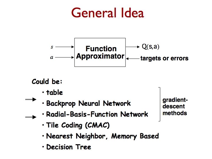
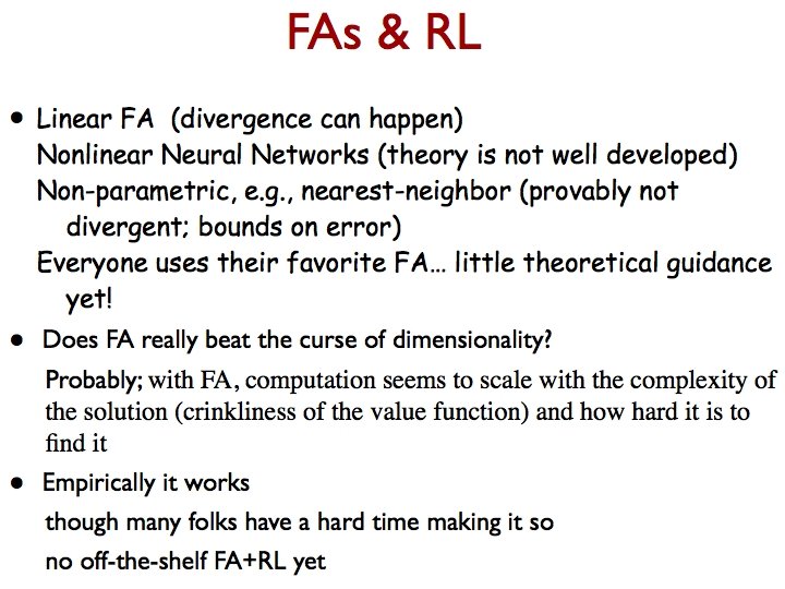
So far… • All Lookup tables – Asymptotic (& rates in some cases) convergence • Practical Problems (like very large state spaces; scaling!) – Function Approximation – Sampling Trees

Gradient Descent

Sparse Coding

Sampling Trees Approach

Sparse Sampling Monte-Carlo Sampling UCT (Kocsis & Szepesvari; others) In time independent of size of state space (polynomial in horizon) near-optimal action with high probability in root state (Kearns, Ng, Mansour)

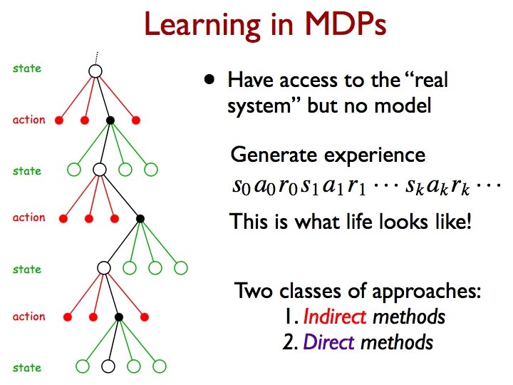
So far… • Basics of RL – Lots of nice results and applications • But crucially given – States – Actions – Rewards • For flexible AI; these are rarely given or easily determined

States? • In many engineering/OR/game problems, this is clear. • In many narrow-domains this might be clear. • But what about for a dog or a person? Or a future android? • Simultaneously – Too many sensors – Too few sensors

Approaches • Bayesian methods / Graphical Models / Relational models / Probabilistic Relational Models – Fruitful endeavors that you have heard much about in this summer school • An alternative approach based on predictions as representations of state – PSRs (Littman, Sutton & Singh; Singh, James & Rudary; Jaeger’s OOMs)

In this part… • Systems that are – Discrete time – Finite observations – Controlled (finite actions) or uncontrolled

POMDPs… actions… at nominal-states at+1 Belief-states are distributions over hidden nominal-states T st st+1 st+2 ot+1 ot+2 O ot observations

Predictions / futures • What is a future? Uncontrolled system: a future is sequence of observations t = o 1 o 2 … o k Controlled system: a future is sequence of observations for a sequence of actions t = a 1 o 1 a 2 o 2 … ak ok • What is a prediction for a future? Uncontrolled system: p(t) = prob(o 1=o 1, …, ok=ok) Controlled system: p(t) = prob(o 1=o 1, …, ok=ok|a 1=a 1, …, ak=ak)

System Dynamics Vector All possible futures! t 1 p(t 1) t 2 t 3 t 4 ti p(ti) There may be 0’s in here… Mathematical construct that IS the system (not a model) Any exact model of a system should be able to generate this vector For both controlled and uncontrolled systems… Lots of constraints on the entries of this vector A “System” is a distribution over all futures…

System Dynamics Matrix t 1 t 2 t 3 t 4 h 1 = p(t 1) h 2 h 3 hj p(t 1|hj) ti p(ti) p(ti|hj) Uncontrolled system: ti=o 1 o 2…ok hj=o 1 o 2…on p(ti|hj) = prob(on+1=o 1, …on+k=ok|o 1 o 2 …on) Controlled system: ti=a 1 o 1…akok hj=a 1 o 1…anon p(ti|hj) = prob(on+1=o 1, …on+k| a 1 o 1…anon, an+1=a 1, …, an+k=ak) tests or experiments… Again, this construct IS the system (not a model)

System Dynamics Matrix t 1 t 2 t 3 t 4 h 1 = p(t 1) h 2 h 3 Only those histories that can happen hj p(t 1|hj) ti p(ti) p(ti|hj) All rows are determined uniquely by the first row Linear dimension of dynamical system is the rank (say N) of its system dynamics matrix (only consider finite rank systems here) Any model must be able to generate this matrix

System Dynamics Matrix Q = {q 1 q 2 … q. N} Core tests t 1 t 2 t 3 t 4 h 1 = p(t 1) h 2 h 3 hj p(t 1|hj) ti p(ti) p(ti|hj) h p(t|h) = p(Q|h)T mt ; note that mt is independent of h ! Prediction for any test is linear combination of the predictions of the core tests p(Q|h) t

nth-order Markov Models all length one tests At most as many unique rows as possible n-length histories (lets say K) t 1 t 2 t 3 t 4 h 1 = p(t 1) h 2 Model parameters h 3 hj p(t 1|hj) Unique histories Theorem: All K-history (nth-order) Markov models are dynamical systems of linear-dimension <= K ti p(ti) p(ti|hj)

K-history Markov models… • Theorem: there exist dynamical systems of lineardimension N that cannot be modeled by any finiteorder Markov model Consider a system in which the first observation determines which of two sub-systems is entered…

POMDPs… actions… at nominal-states at+1 Belief-states are distributions over hidden nominal-states T st st+1 st+2 ot+1 ot+2 O ot observations Learning POMDP models from data (EM) does not work very well; almost no applications

POMDPs… • n underlying or nominal-states State representation for any history h (belief-state) b(h) [a probability distribution over nominal-states] • Update parameters – Transition probabilities Ta (one for every a); Observation probabilities Oao; (for every a, o) Initial belief state b(h 0) • b(hao) = b(h)Ta. Oao/Z = b(h) Bao/Z • For t = a 1 o 1…akok; p(t|h) =b(h) Ta 1 Oa 1 o 1…Tak. Oakok = b(h) Bt predictions linear in belief-states

POMDPs h 0 h 1 D = h 2 hj tt 11 tt 22 tt 33 tt 44 p(t b(h 10|h )B 0 t 1) tti i p(ti 0|h b(h )B 0 ti) p(t 1 j|h b(h )Bjt 1) p(tij|h b(h )Bjti) Linear combination with weights b(h 2) of the rows corresponding to the n rows whose belief-states are unit-basis • Theorem: Every POMDP with ‘n’ nominal states is a dynamical system of linear-dimension n

POMDPs h 0 h 1 D = h 2 hj t 1 t 2 t 3 t 4 b(h 0)Bt 1 ti b(h 0)Bti b(hj)Bt 1 b(hj)Bti Theorem: there exist dynamical systems of finite linear-dimension that cannot be modeled by any finite nominal-state POMDP Intuition: POMDP restricted to positive linear combinations…

PSRs t 1 t 2 h 1 = p(t 1) h 2 h 3 hj q 1 q 2. . . q N t 3 t 4 p(t 1|hj) ti p(ti) p(ti|hj) Core tests Q = {q 1 q 2. . . q. N} State representation: p(Q|h) = [p(q 1|h). . . p(q. N|h)]

t 1 t 2 t 3 t 4 PSRs h 1 = p(t ) 1 h 2 h 3 hj ti p(Q|h 1)m p(Q|hj)m p(t 1|hj) p(Q|h)mt h hao t ? p(Q|h) is a sufficient statistic for history h

Updating Linear PSRs • Update core test qi on taking action a and observing o in history h • Note: one only needs parameters for the one step extensions to the core tests! m’s can have negative entries!! model parameters

Update Parameters… All 1 -step extensions of core tests All 1 -step tests a 1 o 1 aj o j t 1 t 2 h 1 = p(t 1) h 2 h 3 hj p(t 1|hj) q 1 q 2. . . q N t 3 t 4 ti a 1 o 1 q 1 aj o j q N

Linear PSRs • Theorem: Every discrete-time dynamical system of linear-dimension ‘n’ is equivalent to a linear PSR with ‘n’ core tests

Actions…

Actions? • MDPs: Assume uniform time-scale of actions • We can clearly plan at all kinds of temporal scales including variable temporal scales simultaneously • Macro-Actions – Options (Sutton, Precup & Singh; picked up by many others) – MAXQ (Dietterich; picked up by many others) – HAMs (Parr & Russell; picked up by others)

Options A generalization of actions to include courses of action Option execution is assumed to be call-and-return Example: docking I : all states in which charger is in sight hand-crafted controller : terminate when docked or charger not visible Options can take variable number of steps

Rooms Example 4 rooms 4 hallways ROOM HALLWAYS 4 unreliable primitive actions up left O 1 right Fail 33% of the time down G? O 2 G? 8 multi-step options (to each room's 2 hallways) Given goal location, quickly plan shortest route Goal states are given a terminal value of 1 All rewards zero =. 9

Options define a Semi-Markov Decison Process (SMDP) Discrete time Homogeneous discount Continuous time Discrete events Interval-dependent discount Discrete time Overlaid discrete events Interval-dependent discount A discrete-time SMDP overlaid on an MDP Can be analyzed at either level

MDP + Options = SMDP Theorem: For any MDP, and any set of options, the decision process that chooses among the options, executing each to termination, is an SMDP. Thus all Bellman equations and DP results extend for value functions over options and models of options (cf. SMDP theory).

What does the SMDP connection give us? A theoretical fondation for what we really need! But the most interesting issues are beyond SMDPs. . .

Models of Options Knowing how an option is executed is not enough for reasoning about it, or planning with it. We need information about its consequences This form follows from SMDP theory. Such models can be used interchangeably with models of primitive actions in Bellman equations.

Room Example 4 rooms 4 hallways ROOM HALLWAYS 4 unreliable primitive actions up left O 1 right Fail 33% of the time down G? O 2 G? 8 multi-step options (to each room's 2 hallways) Given goal location, quickly plan shortest route Goal states are given a terminal value of 1 All rewards zero =. 9

Example: Synchronous Value Iteration Generalized to Options

Rooms Example

Example with Goal Subgoal both primitive actions and options

What does the SMDP connection give us? A theoretical foundation for what we really need! But the most interesting issues are beyond SMDPs. . .

Advantages of Dual MDP/SMDP View At the SMDP level Compute value functions and policies over options with the benefit of increased speed / flexibility At the MDP level Learn how to execute an option for achieving a given goal Between the MDP and SMDP level Improve over existing options (e. g. by terminating early) Learn about the effects of several options in parallel, without executing them to termination

Between MDPs and SMDPs • Termination Improvement Improving the value function by changing the termination conditions of options • Intra-Option Learning the values of options in parallel, without executing them to termination Learning the models of options in parallel, without executing them to termination • Tasks and Subgoals Learning the policies inside the options

Termination Improvement Idea: We can do better by sometimes interrupting ongoing options - forcing them to terminate before says to

Landmarks Task: navigate from S to G as fast as possible 4 primitive actions, for taking tiny steps up, down, left, right 7 controllers for going straight to each one of the landmarks, from within a circular region where the landmark is visible In this task, planning at the level of primitive actions is computationally intractable, we need the controllers

Termination Improvement for Landmarks Task Allowing early termination based on models improves the value function at no additional cost!

Intra-Option Learning Methods for Markov Options Idea: take advantage of each fragment of experience SMDP Q-learning: • execute option to termination, keeping track of reward along the way • at the end, update only the option taken, based on reward and value of state in which option terminates Intra-option Q-learning: • after each primitive action, update all the options that could have taken that action, based on the reward and the expected value from the next state on Proven to converge to correct values, under same assumptions as 1 -step Q-learning

Intra-Option Learning Methods for Markov Options Idea: take advantage of each fragment of experience SMDP Learning: execute option to termination, then update only the Intra-Option Learning: after each primitive action, update all the options that could have taken that action Proven to converge to correct values, under same assumptions as 1 -step Q-learning option taken

Summary: Benefits of Options • Transfer – Solutions to sub-tasks can be saved and reused – Domain knowledge can be provided as options and subgoals • Potentially much faster learning and planning – By representing action at an appropriate temporal scale • Models of options are a form of knowledge representation – Expressive – Clear – Suitable for learning and planning • Much more to learn than just one policy, one set of values – A framework for “constructivism” – for finding models of the world that are useful for rapid planning and learning

Rewards…

Rewards? • Where do rewards come from? – In narrow engineering tasks this may be clear – But even in such tasks, it need not be (Andrew Ng) • Internal rewards! – Breaking the confound (Singh, Lewis, Sorg, Barto) – Specific internal rewards • Prediction errors (Schmidhuber & many others) • Surprise/Novelty/Curiosity (Oudeyer, Kaplan, Schmidhuber, Singh, Barto & many others)

Power and generality of RL One reason RL is powerful • Reward functions permit specification of what the agent is to do, independently of how it is to do it • RL theory and algorithms are insensitive to the source of rewards – hence their generality Cog. Sci: This generality also defers questions about the nature of reward functions: RL is focused on post-reward algorithms ML/AI: This generality comes at the cost of a detrimental preferences-parameters confound

Preferences-Parameters Confound • The reward function confounds two roles simultaneously in RL agents 1. (Preferences) It expresses the agent-designer’s preferences over behaviors 2. (Parameters) Through the reward hypothesis it expresses the RL agent’s goals/purposes and becomes parameters of actual agent behavior These roles are distinct; there is no apriori reason for them to be confounded

Example - Rewards as Parameters • Q-learning – (Usual) Parameters • Initial Q-value function Q 0: S×A -> scalars • Learning rate, α; Exploration rate, ε – Loop • • Current state st Choose action at (greedy with prob. 1 – ε; random else) Next state st+1; receive reward rt+1 Update: Qt+1(st, at) = (1 - α)Qt(st, at) + α(rt+1 + γ maxb Qt(st+1, b)) Reward function is also a parameter (perhaps the most influential parameter!)

Disentangling the PP Confound • There are two reward functions 1) Agent-designer’s reward U : behavior -> scalar 2) Agent’s reward: RI (in additive form) • Sets up a meta-optimization problem – Agent G(RI; Θ); Environment E; Agent-designer’s U – V(Ri) = E [ U(behavior) | G(RI; Θ) acts in E ] – R*I = arg max V(RI) – (E could be a distribution over environments)

Sanity Check • Theorem: (proof by definition ♪♫♪♬…) Provided the search space of rewards includes the agent-designer’s reward, the agent using the best internal reward can do no worse than the agent using the agent-designer’s reward • Disentangling the PP confound cannot hurt!

Natural Agents • Where do Rewards come from? – Agent designer is evolution – Evolution’s utility function is the fitness function – Natural agents are RL agents • Neuroscience evidence backing this up in terms of dopamine as RL -reward – Evolution designs the natural agent’s reward function. – Agent learns a secondary reward function or value function using RL to adapt to its specific environment. – Two time scales: evolution & within-lifetime

Natural Agents • Reward functions are an important locus of adaptation in adaptive agents; they are a key mechanism for converting distal pressures on fitness into proximal pressures on behavior. • It is possible to precisely formulate this adaptation as a search over possible reward functions, in which reward functions are evaluated in terms of their fitness-conferring abilities Implicit in above: reward is not fitness – reward captures fitness pressures but is simultaneously a locus of knowledge about interactions of environment regularities and agent structure

Computational Experiments

Solving the Meta-Problem • Loop (Select a next reward to explore) – Loop (Sample an environment from distribution over environments) • Initialize agent with selected reward as parameter • Generate behavior and compute fitness/agent-designer’s utility – Average across samples to get value of reward to agent-designer/evolution • Return best reward found • More generally, a mapping from multidimensional agent rewards to scalar value for agent-designer/evolution

Experiment: Fish-or-Bait E: Fixed location for fish and bait A: movement actions, eat, carry A: observes location & food, bait when at those locations & hunger-level & carrying-status Bait can be carried or eaten Fish can be eaten only if bait is carried on agent Eat fish -> not-hungry for 1 step Eat bait -> med-hungry for 1 step else hungry Fitness: F(h) increment of 1. 0 for each fish 0. 04 for each bait eaten

Reward Space Reward features: hunger-level (3 values) Multiple experiments: for varying lifetimes/horizons Lifetime length at which agent has enough time to learn to eat fish with designer’s reward > by 3. 0 Lifetime length at which agent has enough time to learn to eat fish with internal reward

Reward Space Small mitigation effect > by 3. 0 Full mitigation effect

More results Time it takes the best reward at 26, 000 to learn to start to fish

Change in Agent Rewards Agent rewards are not “nice” transformations of the agent-designer’s reward!

ML: The PP Confound • Conjecture: – Stronger Theorem (cartoon form here) For Bounded agents, the best internal reward obtained via solving the meta-optimization problem will strictly outperform the confounded reward. • Corollary: Confounding is fine in unbounded agents. • Internal rewards mitigate agent boundedness – Empirical work thus far with one theoretical result

Mitigation? Increasing Agent-Designer Utility Unbounded agent with confounded reward Bounded agent with best internal reward Bounded agent with confounded reward

Experiment: Foraging E: Worm when eaten disappears. new worm appears at random location A: (actions) movement, eat A: (observations) location, whether it is hungry, not see where worm is unless at worm loc. A: is not-hungry for 1 -step on eating worm Model-based learning agent: builds MDP model from observation experience and always acts greedily Fitness: F(h) increments by one for every worm eaten

Mitigating Agent-State Boundedness • Bound: Agent has limited state information • Contrary to most RL tasks, the agent has to persistently explore (not converge to a policy) • Reward space: linear function of two features – (Real) Inverse-Recency, i. e. , inverse of how long ago did agent execute action last in state – (Binary) Hunger-level

Mitigating Agent-State Boundedness Reward Type βhunger Random 0 Agent-designer 1 Best Agent 0. 0123 Bayes-Optimal βrecency 0 0 0. 999 Asymptotic Agent-Designer Utility per 10, 000 time steps 98 0. 16 754 1543

Experiment: Foraging • Same foraging domain • Agent can see worm’s location (and so no agent state boundedness) • Agent learns an MDP model (recall worm appears in random locations) • Agent can only do depth-limited planning • Separate experiment for each value of depth

Mitigating Depth-Limited Planning

Internal Reward (Lessons so far) 1. 2. 3. 4. 5. 6. RL (and indeed decision-theoretic approaches to AI) suffer from the Preferences-Parameters confound. In fact, there are two reward functions: a) the agent-designer’s reward, and b) the agent’s reward Disentangling the confound creates a specific meta-optimization problem Solving the meta-problem mitigates agent-boundedness The agent’s reward function need not be “nicely” related to the agent-designer’s reward (e. g. , non-monotonic transformations) Good agent rewards are sensitive to details (e. g. , type) of agentboundedness as well as distribution over environments (capturing invariances across environments). Small changes in agent’s reward can lead to large changes in agent behavior and thus large changes in the utility obtained by the agentdesigner.

Distribution over MDPs • MDP = • Beliefs b(θ) • Bayesian Planning (Intractable) • Mean-MDP Planning

Mean-MDP + Reward Bonus Candidates for reward bonus • 1/n (Kolter & Ng ) • 1/√n (MBIE) • Variance of Posterior

Variance of Posterior • Variance of transitions and rewards

Variance of Posterior as Reward Theorem: A (staged version) of the algorithm will follow an ε-optimal policy from its current state on all but a O(1/ε, 1/δ, poly(|S|, |A|)) number of steps with probability at least 1 – δ. In essence, variance-of-posterior based additive internal reward mitigates the limitation of mean-MDP planning.

Hunt-the-Wumpus World

Wumpus Results Parameter Objective Reward / Episode Variance 0. 24 0. 508 1/n 0. 012 0. 293 1/√n 0. 012 0. 291 BOSS K = 20 0. 183 Mean-MDP N/A 0. 266

Random Thought • The focus here has been on inference (and there is tremendous progress) • Often cognitive science tasks require actions. • To the extent that agents were bounded (relative to task? ) the emphasis on inference may be misplaced – Focusing computational resources on good inference may not be best use for good decisionmaking