Reinforcement Learning Overview Introduction Qlearning Exploration vs Exploitation

Reinforcement Learning

Overview Introduction Q-learning Exploration vs. Exploitation Evaluating RL algorithms On-Policy Learning: SARSA

NOTE For this topic, we will refer to the additional textbook Artificial Intelligence: Foundations of Computational Agents (P&M). By David Poole and Alan Mackworth. • Relevant chapter posted on the course schedule page Simpler, clearer coverage, one minor difference in notation you need to be aware of • U(s) => V(s) In the slides, I will use U(s) for consistency with previous lectures

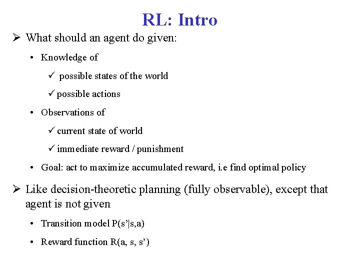
RL: Intro What should an agent do given: • Knowledge of possible states of the world possible actions • Observations of current state of world immediate reward / punishment • Goal: act to maximize accumulated reward, i. e find optimal policy Like decision-theoretic planning (fully observable), except that agent is not given • Transition model P(s’|s, a) • Reward function R(a, s, s’)

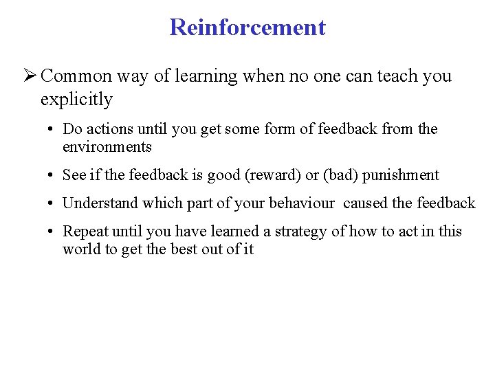
Reinforcement Common way of learning when no one can teach you explicitly • Do actions until you get some form of feedback from the environments • See if the feedback is good (reward) or (bad) punishment • Understand which part of your behaviour caused the feedback • Repeat until you have learned a strategy of how to act in this world to get the best out of it

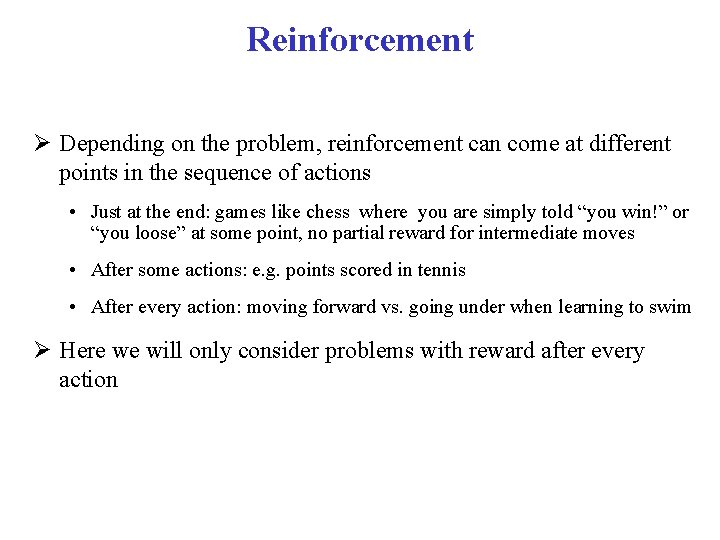
Reinforcement Depending on the problem, reinforcement can come at different points in the sequence of actions • Just at the end: games like chess where you are simply told “you win!” or “you loose” at some point, no partial reward for intermediate moves • After some actions: e. g. points scored in tennis • After every action: moving forward vs. going under when learning to swim Here we will only consider problems with reward after every action

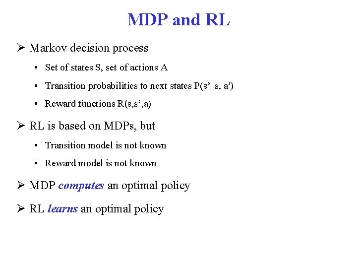
MDP and RL Markov decision process • Set of states S, set of actions A • Transition probabilities to next states P(s’| s, a′) • Reward functions R(s, s’, a) RL is based on MDPs, but • Transition model is not known • Reward model is not known MDP computes an optimal policy RL learns an optimal policy

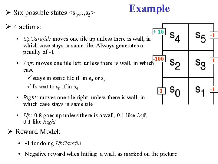
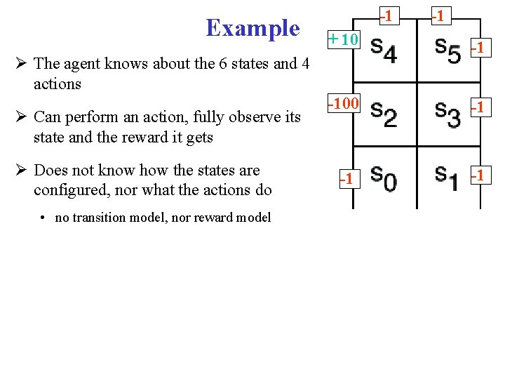
Six possible states <s 0, . . , s 5> Example 4 actions: + 10 • Up. Careful: moves one tile up unless there is wall, in which case stays in same tile. Always generates a penalty of -1 -100 • Left: moves one tile left unless there is wall, in which case stays in same tile if in s 0 or s 2 Is sent to s 0 if in s 4 -1 • Right: moves one tile right unless there is wall, in which case stays in same tile • Up: 0. 8 goes up unless there is a wall, 0. 1 like Left, 0. 1 like Right Reward Model: • -1 for doing Up. Careful • Negative reward when hitting a wall, as marked on the picture -1 -1 -1

Example -1 + 10 -1 -100 -1 -1 -1 The agent knows about the 6 states and 4 actions Can perform an action, fully observe its state and the reward it gets Does not know how the states are configured, nor what the actions do • no transition model, nor reward model -1

Search-Based Approaches to RL Policy Search a) Start with an arbitrary policy b) Try it out in the world (evaluate it) c) Improve it (stochastic local search) d) Repeat from (b) until happy This is called evolutionary algorithm as the agent is evaluated as a whole, based on how it survives Problems with evolutionary algorithms • state space can be huge: with n states and m actions there are mn policies • use of experiences is wasteful: cannot directly take into account locally good/bad behavior, since policies are evaluated as a whole

Overview Introduction Q-learning Exploration vs. Exploitation Evaluating RL algorithms On-Policy Learning: SARSA

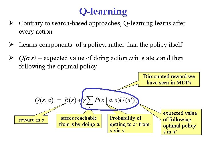
Q-learning Contrary to search-based approaches, Q-learning learns after every action Learns components of a policy, rather than the policy itself Q(a, s) = expected value of doing action a in state s and then following the optimal policy Discounted reward we have seen in MDPs reward in s states reachable from s by doing a Probability of getting to s’ from s via a expected value of following optimal policy л in s’

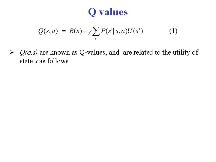
Q values Q(a, s) are known as Q-values, and are related to the utility of state s as follows

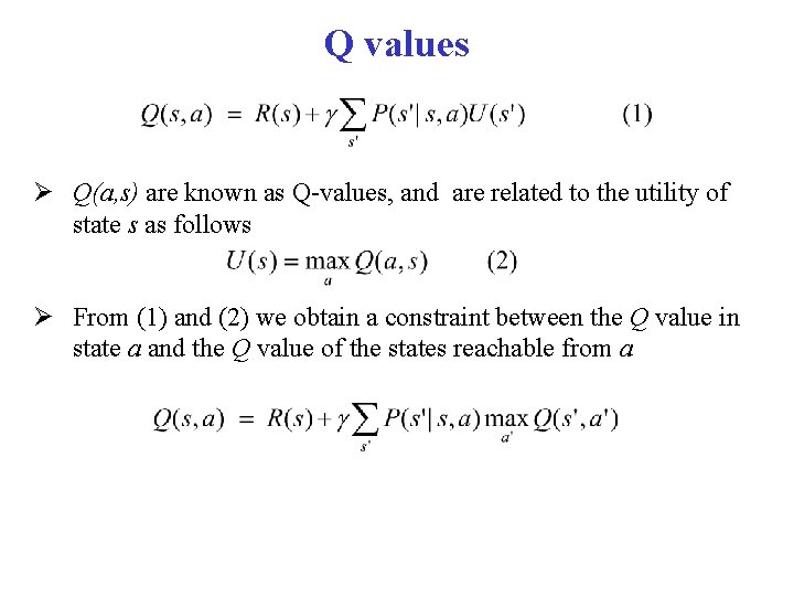
Q values Q(a, s) are known as Q-values, and are related to the utility of state s as follows From (1) and (2) we obtain a constraint between the Q value in state a and the Q value of the states reachable from a

Q values s 0 s 1 … sk a 0 Q[s 0, a 0] Q[s 1, a 0] …. Q[sk, a 0] a 1 Q[s 0, a 1] Q[s 1, a 1] … Q[sk, a 1] … …. … an Q[s 0, an] Q[s 1, an] …. Q[sk, an] Once the agent has a complete Q-function, it knows how to act in every state By learning what to do in each state, rather then the complete policy as in search based methods, learning becomes linear rather than exponential in the number of states But how to learn the Q-values?

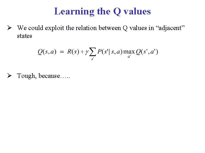
Learning the Q values We could exploit the relation between Q values in “adjacent” states Tough, because…. .

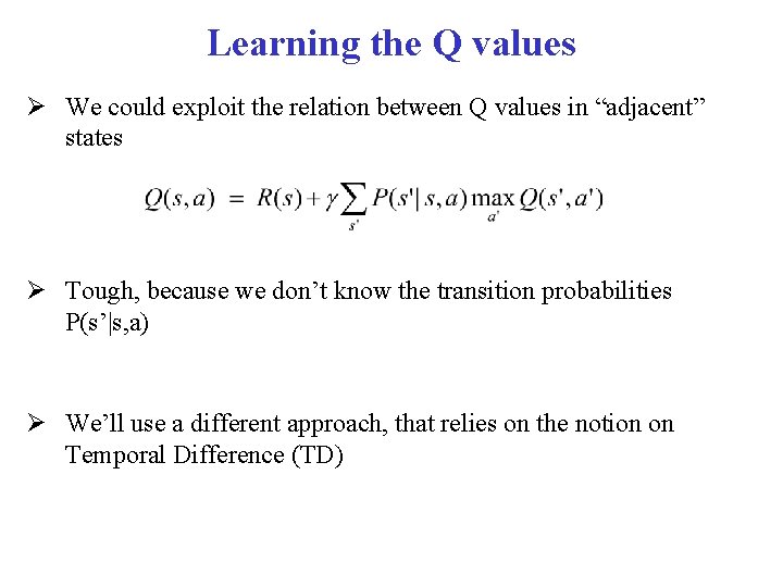
Learning the Q values We could exploit the relation between Q values in “adjacent” states Tough, because we don’t know the transition probabilities P(s’|s, a) We’ll use a different approach, that relies on the notion on Temporal Difference (TD)

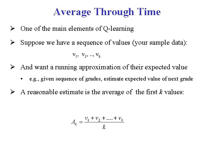
Average Through Time One of the main elements of Q-learning Suppose we have a sequence of values (your sample data): v 1, v 2, . . , vk And want a running approximation of their expected value • e. g. , given sequence of grades, estimate expected value of next grade A reasonable estimate is the average of the first k values:

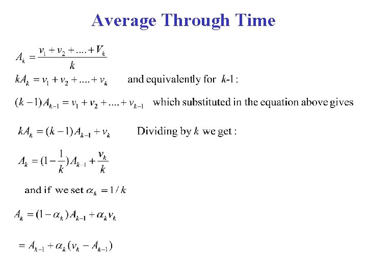
Average Through Time

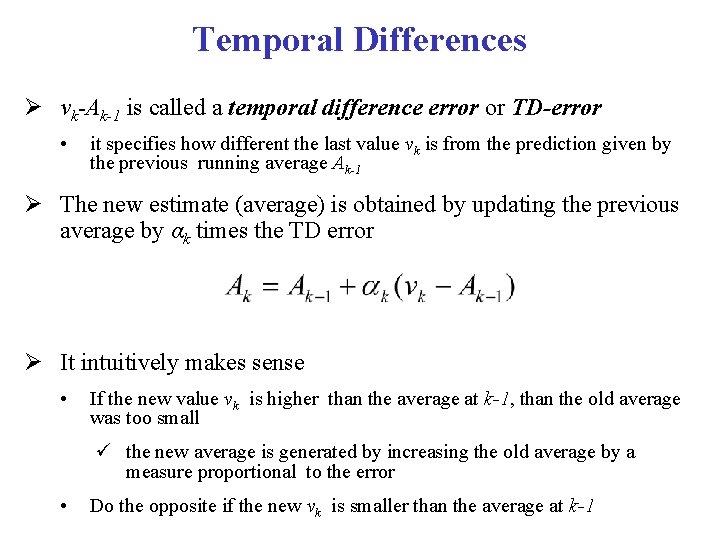
Temporal Differences vk-Ak-1 is called a temporal difference error or TD-error • it specifies how different the last value vk is from the prediction given by the previous running average Ak-1 The new estimate (average) is obtained by updating the previous average by αk times the TD error It intuitively makes sense • If the new value vk is higher than the average at k-1, than the old average was too small the new average is generated by increasing the old average by a measure proportional to the error • Do the opposite if the new vk is smaller than the average at k-1

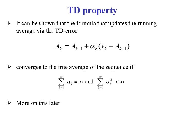
TD property It can be shown that the formula that updates the running average via the TD-error converges to the true average of the sequence if More on this later

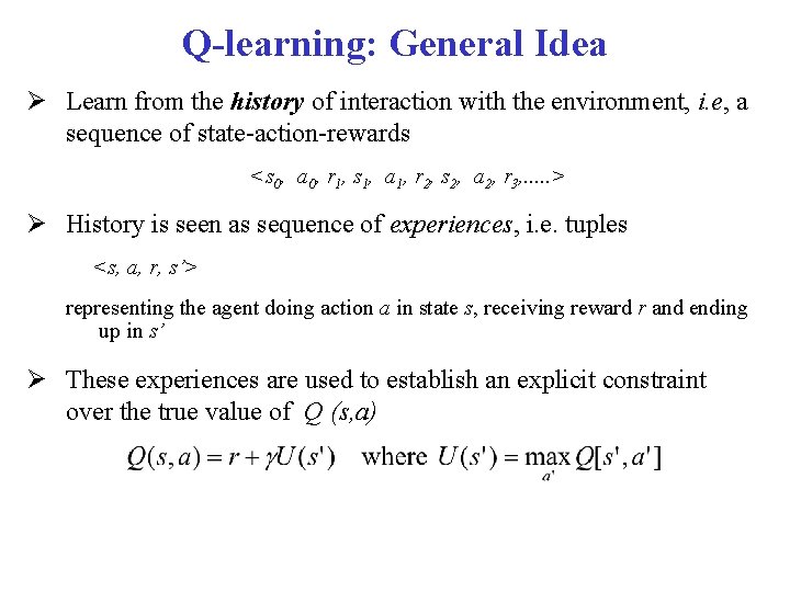
Q-learning: General Idea Learn from the history of interaction with the environment, i. e, a sequence of state-action-rewards <s 0, a 0, r 1, s 1, a 1, r 2, s 2, a 2, r 3, . . . > History is seen as sequence of experiences, i. e. tuples <s, a, r, s’> representing the agent doing action a in state s, receiving reward r and ending up in s’ These experiences are used to establish an explicit constraint over the true value of Q (s, a)

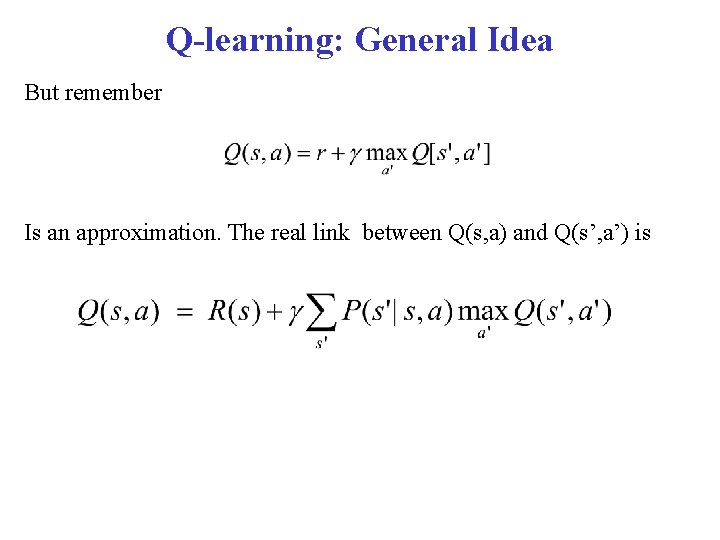
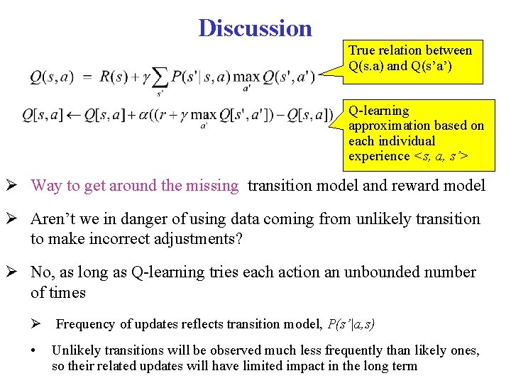
Q-learning: General Idea But remember Is an approximation. The real link between Q(s, a) and Q(s’, a’) is

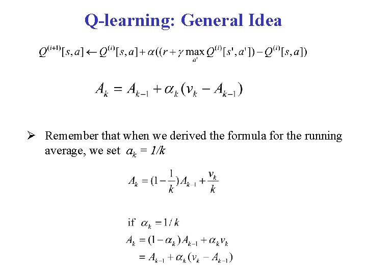
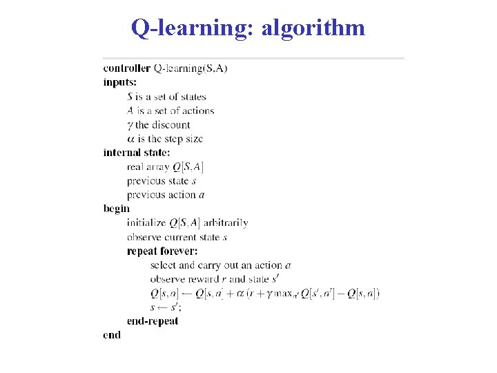
Q-learning: General Idea Store Q[S, A], for every state S and action A in the world Start with arbitrary estimates in Q (0)[S, A], Update them by using experiences • Each experience <s, a, r, s’> provides one data point on the actual value of Q[s, a] current estimated value of Q[s’, a’], where s’ is the state the agent arrives to in the current experience This is used in the TD formula updated estimated value of Q[s, a] current value of current estimated Q[s, a] value of Q[s, a] Datapoint derived from <s, a, r, s’>

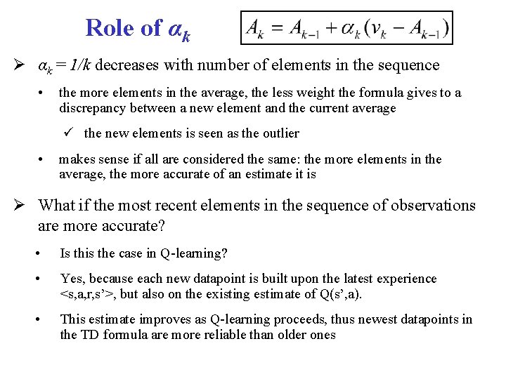
Q-learning: General Idea Remember that when we derived the formula for the running average, we set ak = 1/k

Role of αk = 1/k decreases with number of elements in the sequence • the more elements in the average, the less weight the formula gives to a discrepancy between a new element and the current average the new elements is seen as the outlier • makes sense if all are considered the same: the more elements in the average, the more accurate of an estimate it is What if the most recent elements in the sequence of observations are more accurate? • Is this the case in Q-learning? • Yes, because each new datapoint is built upon the latest experience <s, a, r, s’>, but also on the existing estimate of Q(s’, a). • This estimate improves as Q-learning proceeds, thus newest datapoints in the TD formula are more reliable than older ones

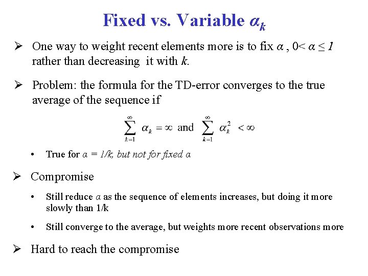
Fixed vs. Variable αk One way to weight recent elements more is to fix α , 0< α ≤ 1 rather than decreasing it with k. Problem: the formula for the TD-error converges to the true average of the sequence if • True for α = 1/k, but not for fixed α Compromise • Still reduce α as the sequence of elements increases, but doing it more slowly than 1/k • Still converge to the average, but weights more recent observations more Hard to reach the compromise

Q-learning: algorithm

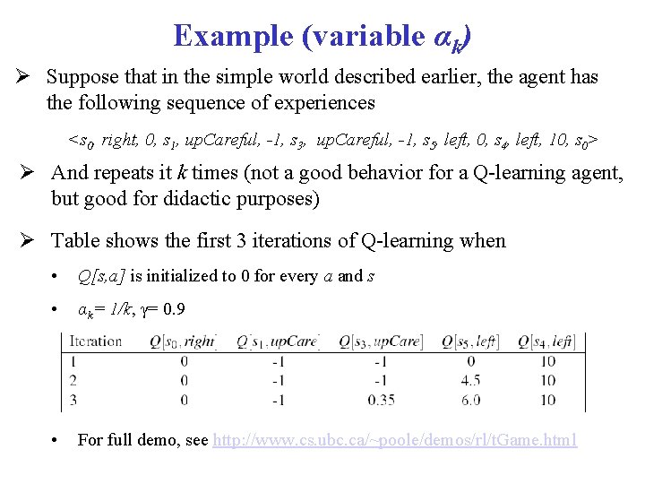
Example (variable αk) Suppose that in the simple world described earlier, the agent has the following sequence of experiences <s 0, right, 0, s 1, up. Careful, -1, s 3, up. Careful, -1, s 5, left, 0, s 4, left, 10, s 0> And repeats it k times (not a good behavior for a Q-learning agent, but good for didactic purposes) Table shows the first 3 iterations of Q-learning when • Q[s, a] is initialized to 0 for every a and s • αk= 1/k, γ= 0. 9 • For full demo, see http: //www. cs. ubc. ca/~poole/demos/rl/t. Game. html

-1 + 10 k=1 Q[s, a] up. Careful Left Right Up s 0 0 0 s 1 0 0 s 2 0 0 s 3 0 0 s 4 0 0 s 5 0 0 -100 -1 -1 -1 Only immediate rewards are included in the update in this first pass

-1 -1 + 10 k=1 k=2 Q[s, a] up. Careful Left Right Up s 0 0 0 s 1 -1 0 0 0 s 2 0 0 s 3 -1 0 0 0 s 4 0 10 0 0 s 5 0 0 -100 -1 1 step backup from previous positive reward in s 4 -1 -1 -1

-1 -1 + 10 k=1 k=3 Q[s, a] up. Careful Left Right Up s 0 0 0 s 1 -1 0 0 0 s 2 0 0 s 3 -1 0 0 0 s 4 0 10 0 0 s 5 0 4. 5 0 0 -100 -1 The effect of the positive reward in s 4 is felt two steps earlier at the 3 rd iteration -1 -1 -1

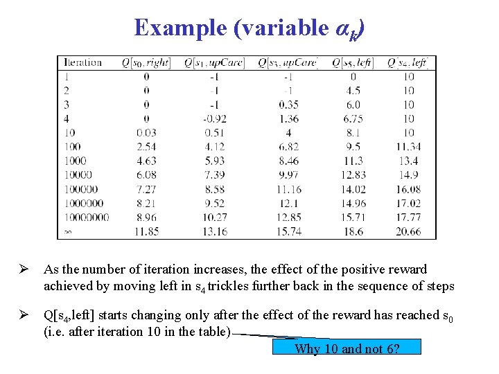
Example (variable αk) As the number of iteration increases, the effect of the positive reward achieved by moving left in s 4 trickles further back in the sequence of steps Q[s 4, left] starts changing only after the effect of the reward has reached s 0 (i. e. after iteration 10 in the table) Why 10 and not 6?

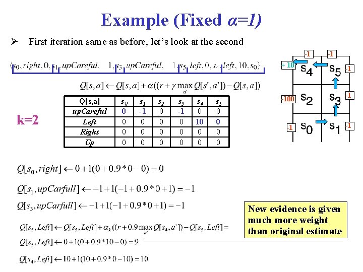
Example (Fixed α=1) First iteration same as before, let’s look at the second -1 -1 + 10 k=2 Q[s, a] up. Careful Left Right Up s 0 0 0 s 1 -1 0 0 0 s 2 0 0 s 3 -1 0 0 0 s 4 0 10 0 0 s 5 0 0 -100 -1 New evidence is given much more weight than original estimate -1 -1 -1

-1 -1 + 10 k=1 k=3 Q[s, a] up. Careful Left Right Up s 0 0 0 s 1 -1 0 0 0 s 2 0 0 s 3 -1 0 0 0 s 4 0 10 0 0 s 5 0 9 0 0 -100 -1 Same here No change from previous iteration, as all the reward from the step ahead was included there -1 -1 -1

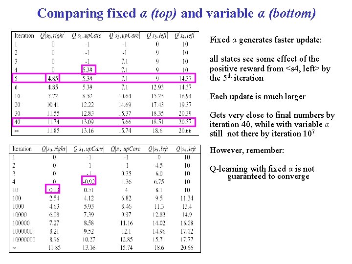
Comparing fixed α (top) and variable α (bottom) Fixed α generates faster update: all states see some effect of the positive reward from <s 4, left> by the 5 th iteration Each update is much larger Gets very close to final numbers by iteration 40, while with variable α still not there by iteration 107 However, remember: Q-learning with fixed α is not guaranteed to converge

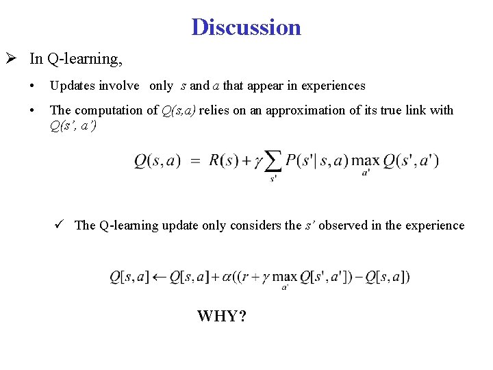
Discussion In Q-learning, • Updates involve only s and a that appear in experiences • The computation of Q(s, a) relies on an approximation of its true link with Q(s’, a’) The Q-learning update only considers the s’ observed in the experience WHY?

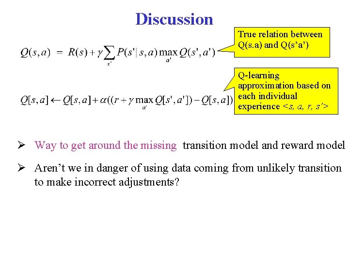
Discussion True relation between Q(s. a) and Q(s’a’) Q-learning approximation based on each individual experience <s, a, r, s’> Way to get around the missing transition model and reward model Aren’t we in danger of using data coming from unlikely transition to make incorrect adjustments?

Discussion True relation between Q(s. a) and Q(s’a’) Q-learning approximation based on each individual experience <s, a, s’> Way to get around the missing transition model and reward model Aren’t we in danger of using data coming from unlikely transition to make incorrect adjustments? No, as long as Q-learning tries each action an unbounded number of times Frequency of updates reflects transition model, P(s’|a, s) • Unlikely transitions will be observed much less frequently than likely ones, so their related updates will have limited impact in the long term

Q-learning learns an optimal policy no matter which actions are selected in each state Q-learning is an off-policy method because it learns an optimal policy no matter which policy the agent is actually following It is also a model-free method, because it does not need to learn an explicit transition model for the environment in order to find the optimal policy • The environment provides the connections between neighboring states in the form of observed transitions