Reinforcement Learning Methods for Military Applications Malcolm Strens

Reinforcement Learning Methods for Military Applications Malcolm Strens Centre for Robotics and Machine Vision Future Systems Technology Division Defence Evaluation & Research Agency U. K. 19 February 2001 © British Crown Copyright, 2001

RL & Simulation n Trial-and-error in a real system is expensive – learn with a cheap model (e. g. CMU autonomous helicopter) – or. . . – learn with a very cheap model (a high fidelity simulation) – analogous to human learning in a flight simulator n Why is RL now viable for application? – most theory developed in last 12 years – computers have got faster – simulation has improved

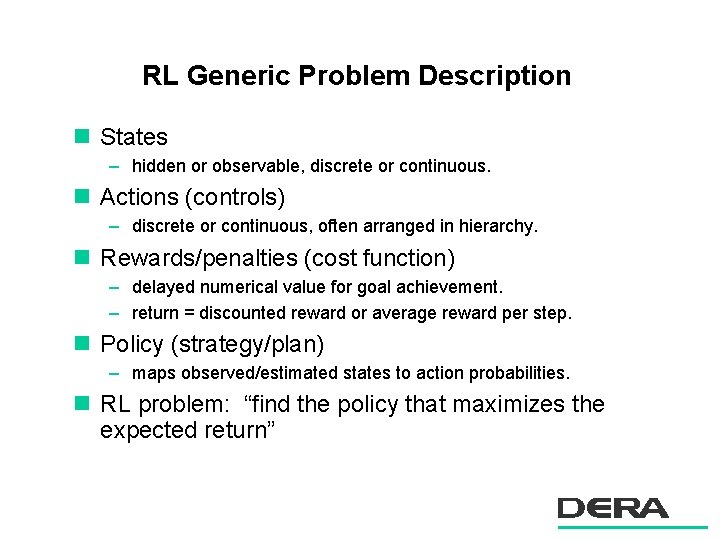
RL Generic Problem Description n States – hidden or observable, discrete or continuous. n Actions (controls) – discrete or continuous, often arranged in hierarchy. n Rewards/penalties (cost function) – delayed numerical value for goal achievement. – return = discounted reward or average reward per step. n Policy (strategy/plan) – maps observed/estimated states to action probabilities. n RL problem: “find the policy that maximizes the expected return”

Existing applications of RL n Game-playing – backgammon, chess etc. – learn from scratch by simulation (win = reward) n Network routing and channel allocation – maximize throughput n Elevator scheduling – minimize average wait time n Traffic light scheduling – minimize average journey time n Robotic control – learning balance and coordination in walking, juggling robots – nonlinear flight controllers for aircraft

Characteristics of problems amenable to RL solution n Autonomous/automatic control & decision-making n Interaction (outputs affect subsequent inputs) n Stochasticity – different consequences each time an action is taken – e. g. non-deterministic behavior of an opponent n Decision-making over time – a sequence of actions over a period of time leads to reward – i. e. planning n Why not use standard optimization methods? – – e. g. genetic algorithms, gradient descent, heuristic search because the cost function is stochastic because there is hidden state because temporal reasoning is essential

Potential military applications of RL: examples n Autonomous decision-making over time – – guidance against reacting target real-time mission/route planning and obstacle avoidance trajectory optimization in changing environment sensor control & dynamic resource allocation n Automatic decision-making – rapid reaction • electronic warfare – low-level control • flight control for UAVs (especially micro-UAVs) • coordination for legged robots n Logistic planning – resource allocation – scheduling

4 current approaches to the RL problem n Value-function approximation methods – estimate the discounted return for every (state, action) – actor-critic methods (e. g. TD-Gammon) n Estimate a working model – estimate a model that explains the observations – solve for optimal behavior in this model – full Bayesian treatment (intractable) would provide convergence and robustness guarantees – certainty-equivalence methods tractable but unreliable – the eventual winner in 20 dimensions+ ? n Direct policy search – apply stochastic optimization in a parameterized space of policies – effective up to at least 12 dimensions (see pursuer-evader results) n Policy gradient ascent – policy search using a gradient estimate

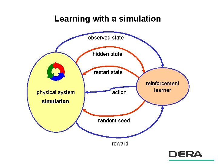
Learning with a simulation observed state hidden state restart state physical system action simulation random seed reward reinforcement learner

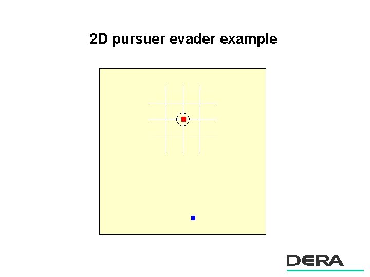
2 D pursuer evader example

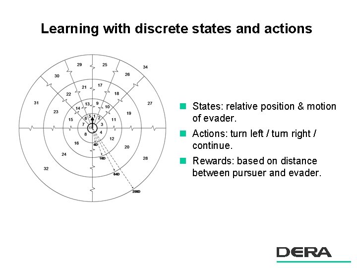
Learning with discrete states and actions n States: relative position & motion of evader. n Actions: turn left / turn right / continue. n Rewards: based on distance between pursuer and evader.

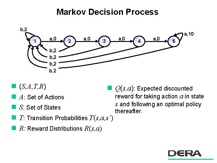
Markov Decision Process b, 2 1 a, 0 2 a, 0 3 a, 0 4 a, 0 a, 10 5 b, 2 n n n (S, A, T, R) n Q(s, a): Expected discounted reward for taking action a in state A: Set of Actions s and following an optimal policy S: Set of States thereafter. T: Transition Probabilities T(s, a, s’) R: Reward Distributions R(s, a)

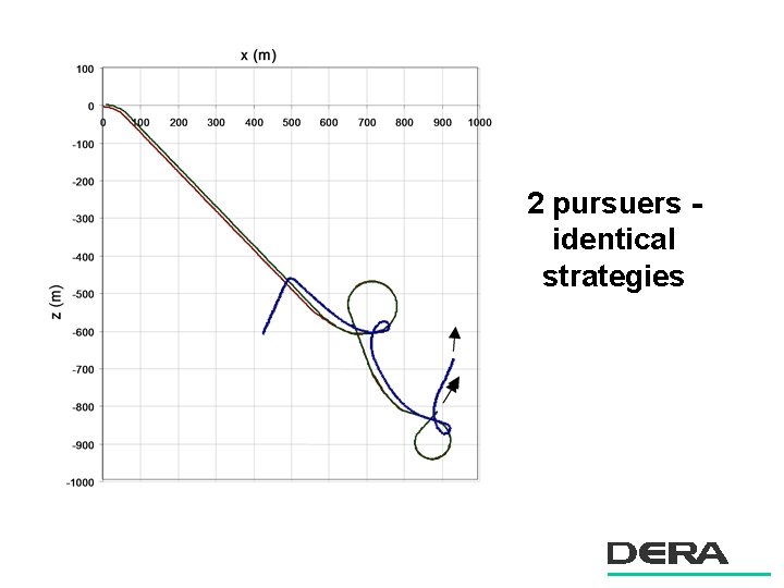
2 pursuers identical strategies

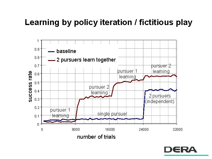
Learning by policy iteration / fictitious play 1 0. 9 baseline 0. 8 2 pursuers learn together pursuer 2 learning success rate 0. 7 pursuer 1 learning 0. 6 0. 5 pursuer 2 learning 0. 4 0. 3 0. 2 pursuer 1 learning 0. 1 2 pursuers (independent) single pursuer 0 0 8000 16000 number of trials 24000 32000

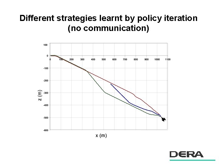
Different strategies learnt by policy iteration (no communication)

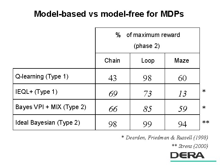
Model-based vs model-free for MDPs % of maximum reward (phase 2) Chain Loop Maze Q-learning (Type 1) 43 98 60 IEQL+ (Type 1) 69 73 13 * Bayes VPI + MIX (Type 2) 66 85 59 * Ideal Bayesian (Type 2) 98 99 94 ** * Dearden, Friedman & Russell (1998) ** Strens (2000)

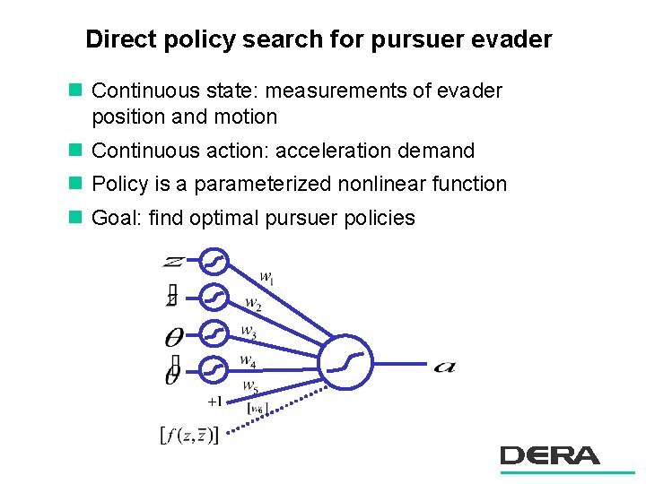
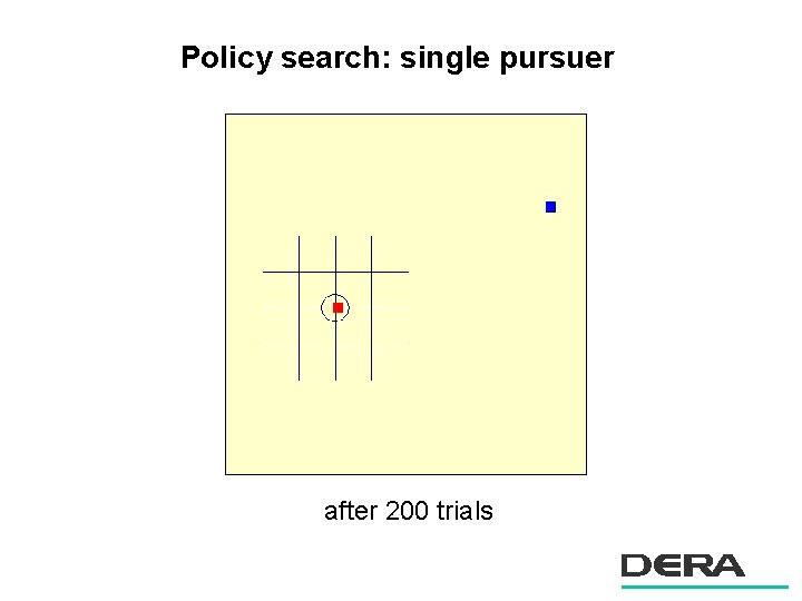
Direct policy search for pursuer evader n Continuous state: measurements of evader position and motion n Continuous action: acceleration demand n Policy is a parameterized nonlinear function n Goal: find optimal pursuer policies

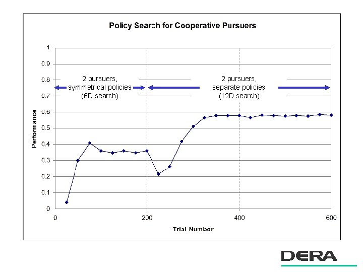
2 pursuers, symmetrical policies (6 D search) 2 pursuers, separate policies (12 D search)

Policy search: single pursuer after 200 trials

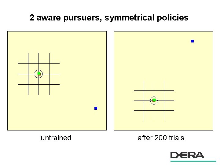
2 aware pursuers, symmetrical policies untrained after 200 trials

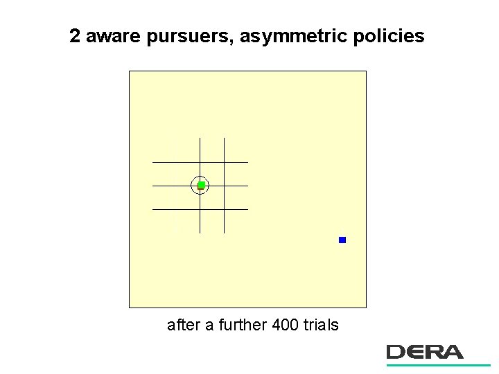
2 aware pursuers, asymmetric policies after a further 400 trials

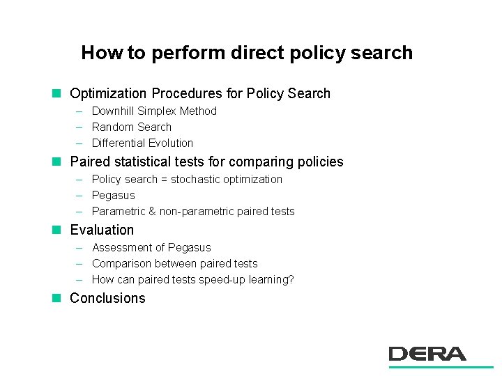
How to perform direct policy search n Optimization Procedures for Policy Search – Downhill Simplex Method – Random Search – Differential Evolution n Paired statistical tests for comparing policies – Policy search = stochastic optimization – Pegasus – Parametric & non-parametric paired tests n Evaluation – Assessment of Pegasus – Comparison between paired tests – How can paired tests speed-up learning? n Conclusions

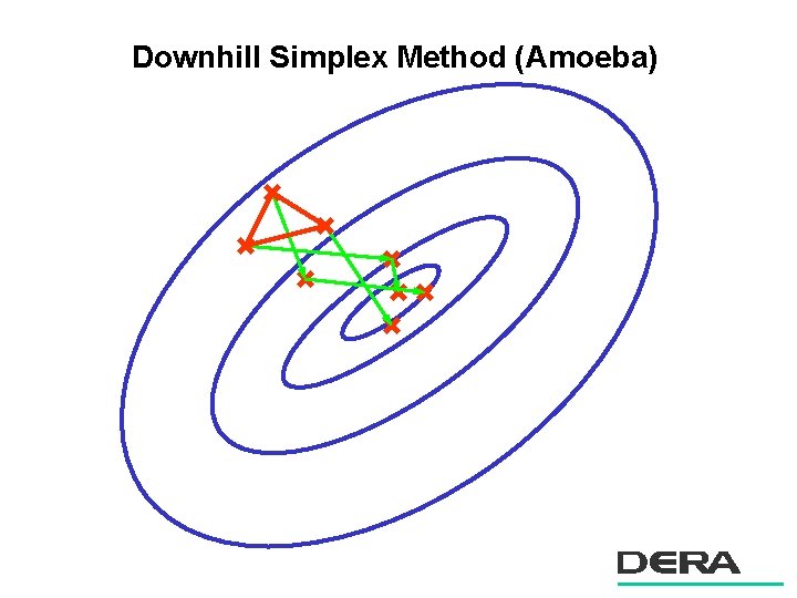
Downhill Simplex Method (Amoeba)

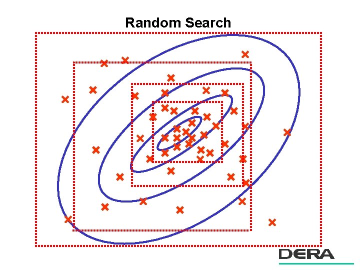
Random Search

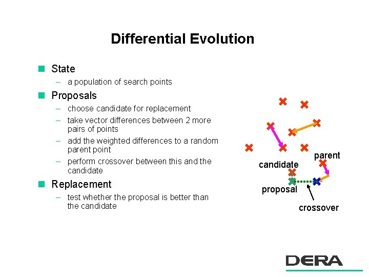
Differential Evolution n State – a population of search points n Proposals – choose candidate for replacement – take vector differences between 2 more pairs of points – add the weighted differences to a random parent point – perform crossover between this and the candidate n Replacement – test whether the proposal is better than the candidate parent proposal crossover

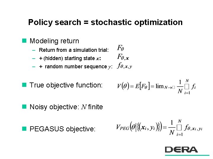
Policy search = stochastic optimization n Modeling return – Return from a simulation trial: – + (hidden) starting state x: – + random number sequence y: n True objective function: n Noisy objective: N finite n PEGASUS objective:

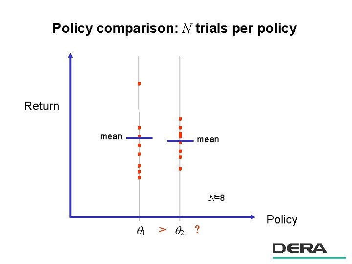
Policy comparison: N trials per policy Return mean N=8 > ? Policy

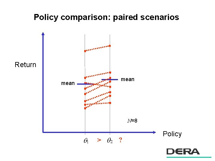
Policy comparison: paired scenarios Return mean N=8 > ? Policy

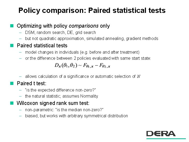
Policy comparison: Paired statistical tests n Optimizing with policy comparisons only – DSM, random search, DE, grid search – but not quadratic approximation, simulated annealing, gradient methods n Paired statistical tests – model changes in individuals (e. g. before and after treatment) – or the difference between 2 policies evaluated with same start state: – allows calculation of a significance or automatic selection of N n Paired t test: – “is the expected difference non-zero? ” – the natural statistic; assumes Normality n Wilcoxon signed rank sum test: – non-parametric: “is the median non-zero? ” – biased, but works with arbitrary symmetrical distribution

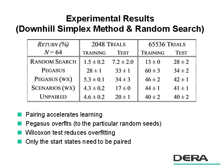
Experimental Results (Downhill Simplex Method & Random Search) n n Pairing accelerates learning Pegasus overfits (to the particular random seeds) Wilcoxon test reduces overfitting Only the start states need to be paired

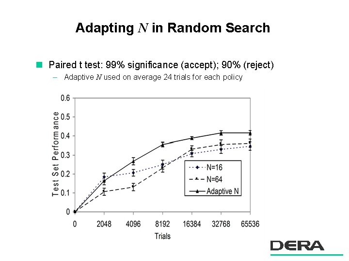
Adapting N in Random Search n Paired t test: 99% significance (accept); 90% (reject) – Adaptive N used on average 24 trials for each policy

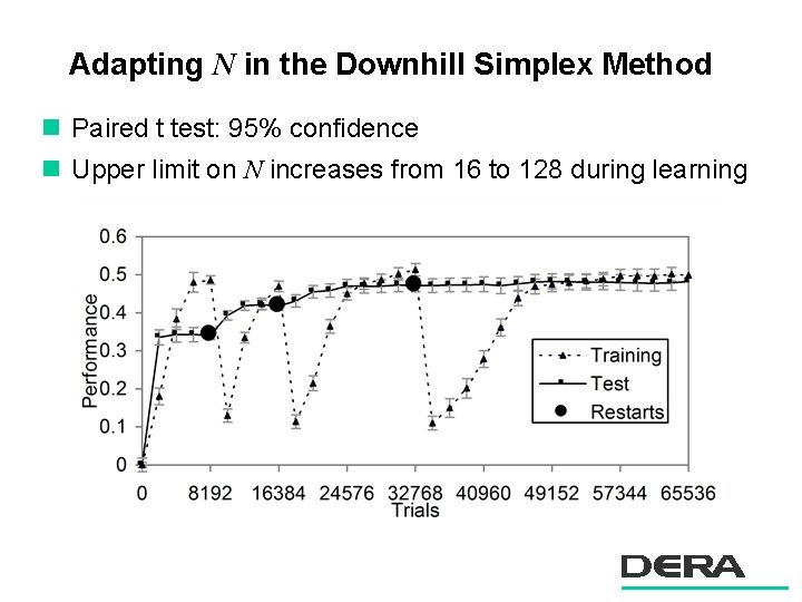
Adapting N in the Downhill Simplex Method n Paired t test: 95% confidence n Upper limit on N increases from 16 to 128 during learning

Differential Evolution: N=2 n Very small N can be used – because population has an averaging effect – decisions only have to be >50% reliable n With unpaired comparisons: 27% performance n With paired comparisons: 47% performance – different Pegasus scenarios for every comparison n The challenge: find a stochastic optimization procedure that – exploits this population averaging effect – but is more efficient than DE.

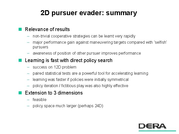
2 D pursuer evader: summary n Relevance of results – non-trivial cooperative strategies can be learnt very rapidly – major performance gain against maneuvering targets compared with ‘selfish’ pursuers – awareness of position of other pursuer improves performance n Learning is fast with direct policy search – success on 12 D problem – paired statistical tests are a powerful tool for accelerating learning – learning was faster if policies were initially symmetrical – policy iteration / fictitious play was also highly effective n Extension to 3 dimensions – feasible – policy space much larger (perhaps 24 D)

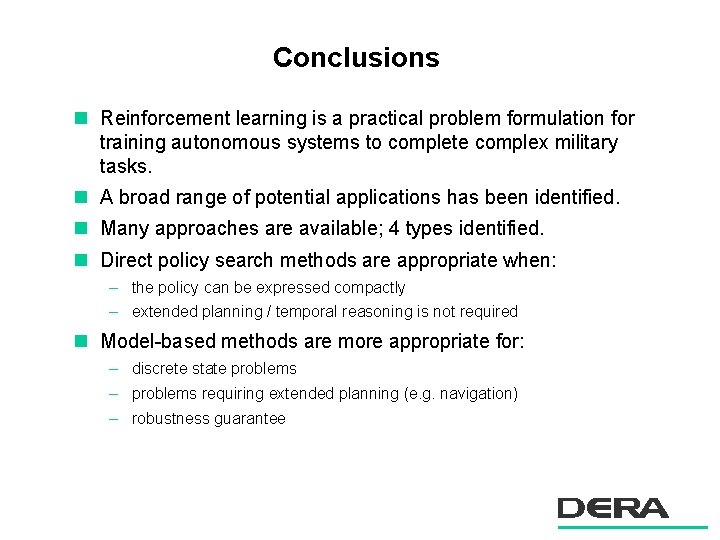
Conclusions n Reinforcement learning is a practical problem formulation for training autonomous systems to complete complex military tasks. n A broad range of potential applications has been identified. n Many approaches are available; 4 types identified. n Direct policy search methods are appropriate when: – the policy can be expressed compactly – extended planning / temporal reasoning is not required n Model-based methods are more appropriate for: – discrete state problems – problems requiring extended planning (e. g. navigation) – robustness guarantee