Reinforcement Learning Learning to Control So far looked


 • Execute actions in environment, observe results. • Learn action policy")


: a.")
 or")


 is enough to determine the State(the state is accessible)")


 Agent makes random runs")


 Uses the value or")
 is reward of")
 = 0. 33 x")

 The key is to")


 approach and Temporal-Difference(TD) approach operate")


 R(s) + γ*maxaf(u, n) u=Ss’(T(s,")
: act randomly in hopes of eventually exploring entire")


: value of action a Reward")
 vs Multiple States")


 • st : State of agent at time")


, p (rt+1 | st")


, p (rt+1")


")
 expected utility? • Problem:")


- Slides: 110
Reinforcement Learning
Learning to Control • So far looked at two models of learning – Supervised: Classification, Regression, etc. – Unsupervised: Clustering, etc. • How did you learn to cycle? – Neither of the above – Trial and error! – Falling down hurts! Intro to RL 2
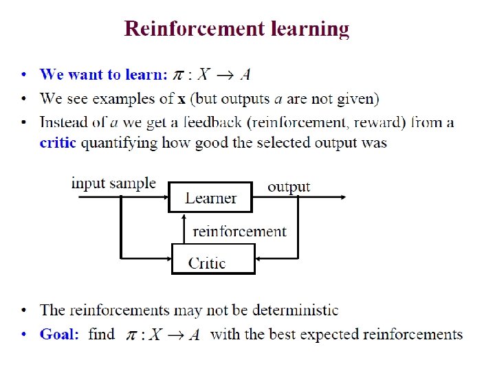
What is Reinforcement Learning? • Learning from interaction • Goal-oriented learning • Learning about, from, and while interacting with an external environment • Learning what to do—how to map situations to actions—so as to maximize a numerical reward signal Reinforcement Learning 3
• Task Reinforcement Learning – Learn how to behave successfully to achieve a goal while interacting with an external environment Learn through experience from trial and error • Examples – Game playing: The agent knows it has won or lost, but it doesn’t know the appropriate action in each state – Control: a traffic system can measure the delay of cars, but not know how to decrease it.
Robot in a room +1 -1 START • • actions: UP, DOWN, LEFT, RIGHT UP 80% 10% move UP move LEFT move RIGHT reward +1 at [4, 3], -1 at [4, 2] reward -0. 04 for each step what’s the strategy to achieve max reward? what if the actions were deterministic?
Reinforcement Learning • Target function is : state action • However… – We have no training examples of form <state, action> – Training examples are of form <<state, action>, reward>
RL Framework Environment evaluation State • • Agent Action Learn from close interaction Stochastic environment Noisy delayed scalar evaluation Maximize a measure of long term performance 8
Not Supervised Learning! Input Output Agent Error • • • Target Very sparse “supervision” No target output provided No error gradient information available Action chooses next state Explore to estimate gradient – Trail and error learning Intro to RL 9
Not Unsupervised Learning Input Agent Activation Evaluation • Sparse “supervision” available • Pattern detection not primary goal Intro to RL 10
Elements of RL Policy Reward Value • • Model of environment Policy: what to do Reward: what is good Value: what is good because it predicts reward Model: what follows what V. Rieser: An Introduction to Reinforcement Learning. C&C, 2005. 11
Elements of RL Agent State Reward Policy Action Environment • Transition model, how action influence states • Reward R, immediate value of state-action transition • Policy , maps states to actions
RL task (restated) • Execute actions in environment, observe results. • Learn action policy : state action that maximizes expected discounted reward E [r(t) + r(t + 1) + 2 r(t + 2) + …] from any starting state in S
RL is learning from interaction
Reinforcement Learning • A trial-and-error learning paradigm – Rewards and Punishments • Not just an algorithm but a new paradigm in itself • Learn about a system – – behaviour – control from minimal feed back • Inspired by behavioural psychology Intro to RL 16
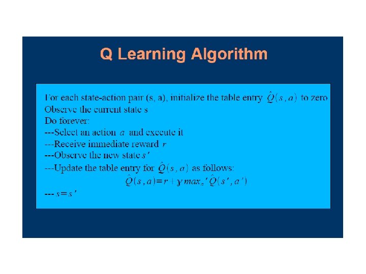
General RL Algorithm i. Initialise learner’s internal state ii. Do forever (!? ): a. Observe current state s b. Choose action a using some evaluation function c. Execute action a d. Let r be immediate reward, s’ new state e. Update internal state based on s, a, r, s’ V. Rieser: An Introduction to Reinforcement Learning. C&C, 2005. 17
To solve the problem mathematically: • Formulate it as Markov Decision Process (MDP) or Partially Observable Markov Decision Process (POMDP) • Maximize the state-value and action-value functions using the Bellmann optimality equation • Use approximations to solve the Bellmann equation such as dynamic programming, Monte Carlo Methods, Temporal-difference Learning. V. Rieser: An Introduction to Reinforcement Learning. C&C, 2005. 18
The Bellmann Equation • Bellmann optimality equation estimates “how good” it is to be in a state s. Vπ(s)=∑aπ(s, a) ∑s’Pss’a[Rss’a+µVπ(s’)] V*(s) = max Qπ*(s, a) Q*(s, a) = ∑Pass´ [Rass´+ max Q*(s´, a´)] “What actions are V. Rieser: An Introductionavailable? ” to Reinforcement Learning. C&C, 2005. 19 [figure (a)] [figure (b)] “How good are those actions? ”
Summary: Key Features of RL ü Learner is not told which actions to take ü Trial-and-Error search ü Possibility of delayed reward (Sacrifice short-term gains for greater longterm gains) ü The need to explore and exploit ü Considers the whole problem of a goal-directed agent interacting with an uncertain environment V. Rieser: An Introduction to Reinforcement Learning. C&C, 2005. 20
RL model • Each percept(e) is enough to determine the State(the state is accessible) • The agent can decompose the Reward component from a percept. • The agent task: to find a optimal policy, mapping states to actions, that maximize longrun measure of the reinforcement • Think of reinforcement as reward • Can be modeled as MDP model!
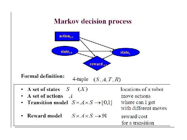
Review of MDP model • MDP model <S, T, A, R> • S– set of states Agent State Action Reward Environment s 0 a 0 r 0 s 1 a 1 r 1 s 2 a 2 r 2 s 3 • A– set of actions • T(s, a, s’) = P(s’|s, a)– the probability of transition from s to s’ given action a • R(s, a)– the expected reward for taking action a in state s
Reinforcement learning • Task Learn how to behave successfully to achieve a goal while interacting with an external environment – Learn via experiences! • Examples – Game playing: player knows whether it win or lose, but not know how to move at each step – Control: a traffic system can measure the delay of cars, but not know how to decrease it.
Model based v. s. Model free approaches • But, we don’t know anything about the environment model—the transition function T(s, a, s’) • Here comes two approaches – Model based approach RL: learn the model, and use it to derive the optimal policy. e. g Adaptive dynamic learning(ADP) approach – Model free approach RL: derive the optimal policy without learning the model. e. g LMS and Temporal difference approach • Which one is better?
Applications of RL • Robot navigation • Adaptive control – Helicopter pilot! • Combinatorial optimization – VLSI placement and routing , elevator dispatching • Game playing – Backgammon – world’s best player! • Computational Neuroscience – Modeling of reward processes Intro to RL 25
Passive Learning – Known Environment
Passive Learning in a Known Environment Passive Learner: A passive learner simply watches the world going by, and tries to learn the utility of being in various states. Another way to think of a passive learner is as an agent with a fixed policy trying to determine its benefits.
Passive Learning in a Known Environment In passive learning, the environment generates state transitions and the agent perceives them. Consider an agent trying to learn the utilities of the states shown below:
Passive Learning in a Known Environment Agent can move {North, East, South, West} Terminate on reading [4, 2] or [4, 3]
Passive Learning in a Known Environment Agent is provided: Mi j = a model given the probability of reaching from state i to state j
Passive Learning in a Known Environment the object is to use this information about rewards to learn the expected utility U(i) associated with each nonterminal state i Utilities can be learned using 3 approaches 1) LMS (least mean squares) 2) ADP (adaptive dynamic programming) 3) TD (temporal difference learning)
Passive Learning in a Known Environment LMS (Least Mean Squares) Agent makes random runs (sequences of random moves) through environment [1, 1]->[1, 2]->[1, 3]->[2, 3]->[3, 3]->[4, 3] = +1 [1, 1]->[2, 1]->[3, 2]->[4, 2] = -1
Passive Learning in a Known Environment LMS Collect statistics on final payoff for each state (eg. when on [2, 3], how often reached +1 vs -1 ? ) Learner computes average for each state Provably converges to true expected value (utilities) (Algorithm on page 602, Figure 20. 3)
Passive Learning in a Known Environment LMS Main Drawback: - slow convergence - it takes the agent well over a 1000 training sequences to get close to the correct value
Passive Learning in a Known Environment ADP (Adaptive Dynamic Programming) Uses the value or policy iteration algorithm to calculate exact utilities of states given an estimated model
Passive Learning in a Known Environment ADP In general: - R(i) is reward of being in state i (often non zero for only a few end states) - Mij is the probability of transition from state i to j
Passive Learning in a Known Environment ADP Consider U(3, 3) = 0. 33 x U(4, 3) + 0. 33 x U(2, 3) + 0. 33 x U(3, 2) = 0. 33 x 1. 0 + 0. 33 x 0. 0886 + 0. 33 x -0. 4430 = 0. 2152
Passive Learning in a Known Environment ADP makes optimal use of the local constraints on utilities of states imposed by the neighborhood structure of the environment somewhat intractable for large state spaces
Passive Learning in a Known Environment TD (Temporal Difference Learning) The key is to use the observed transitions to adjust the values of the observed states so that they agree with the constraint equations
Passive Learning in a Known Environment TD Learning Suppose we observe a transition from state i to state j U(i) = -0. 5 and U(j) = +0. 5 Suggests that we should increase U(i) to make it agree better with it successor Can be achieved using the following updating rule
Passive Learning in a Known Environment TD Learning Performance: Runs “noisier” than LMS but smaller error Deal with observed states during sample runs (Not all instances, unlike ADP)
Passive Learning – Un. Known Environment
Passive Learning in an Unknown Environment Least Mean Square(LMS) approach and Temporal-Difference(TD) approach operate unchanged in an initially unknown environment. Adaptive Dynamic Programming(ADP) approach adds a step that updates an estimated model of the environment.
Passive Learning in an Unknown Environment ADP Approach • The environment model is learned by direct observation of transitions • The environment model M can be updated by keeping track of the percentage of times each state transitions to each of its neighbors
Passive Learning in an Unknown Environment ADP & TD Approaches • The ADP approach and the TD approach are closely related • Both try to make local adjustments to the utility estimates in order to make each state “agree” with its successors
Passive Learning in an Unknown Environment Minor differences : • TD adjusts a state to agree with its observed successor • ADP adjusts the state to agree with all of the successors Important differences : • TD makes a single adjustment per observed transition • ADP makes as many adjustments as it needs to restore consistency between the utility estimates U and the environment model M
Passive Learning in an Unknown Environment To make ADP more efficient : • directly approximate the algorithm for value iteration or policy iteration • prioritized-sweeping heuristic makes adjustments to states whose likely successors have just undergone a large adjustment in their own utility estimates Advantage of the approximate ADP : • efficient in terms of computation • eliminate long value iterations occur in early stage
Active Learning – Unknown Environment
Active Learning in an Unknown Environment An active agent must consider : • what actions to take • what their outcomes may be • how they will affect the rewards received
Active Learning in an Unknown Environment Minor changes to passive learning agent : • environment model now incorporates the probabilities of transitions to other states given a particular action • maximize its expected utility • agent needs a performance element to choose an action at each step
Active Learning in an Unknown Environment Active ADP Approach • need to learn the probability Maij of a transition instead of Mij • the input to the function will include the action taken
Active Learning in an Unknown Environment Active TD Approach • the model acquisition problem for the TD agent is identical to that for the ADP agent • the update rule remains unchanged • the TD algorithm will converge to the same values as ADP as the number of training sequences tends to infinity
Active Reinforcement Learning Now we must decide what actions to take. Optimal policy: Choose action with highest utility value. Is that the right thing to do?
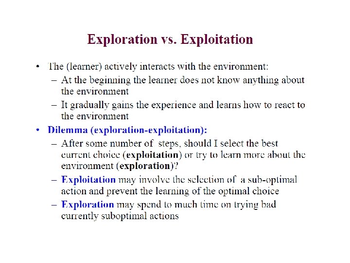
Active Reinforcement Learning No! Sometimes we may get stuck in suboptimal solutions. Exploration vs Exploitation Tradeoff Why is this important? The learned model is not the same as the true environment.
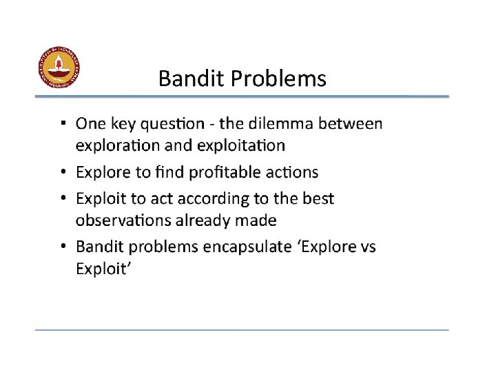
Bandit problem
Explore vs Exploitation: Maximize its reward vs Exploration: Maximize long-term well being.
Simple Solution to the Exploitation/Exploration Problem • Choose a random action once in k times • Otherwise, choose the action with the highest expected utility (k-1 out of k times)
Another Solution --- Combining Exploration and Exploitation U+ (s) R(s) + γ*maxaf(u, n) u=Ss’(T(s, a, s’)*U+(s’)); n=N(a, s) U+ (s) : optimistic estimate of utility N(a, s): number of times action a has been tried. f(u, n): exploration function (idea: returns the value u, if n is large, and values larger than u as n decreases) Example: f(u, n): = if n>navg then u else max(n/navg*u, uavg) navg being the average number of operator applications. Idea f: Utility of states/actions that have not been explored much is increased artificially.
Exploration policy • Wacky approach (exploration): act randomly in hopes of eventually exploring entire environment • Greedy approach (exploitation): act to maximize utility using current estimate • Reasonable balance: act more wacky (exploratory) when agent has little idea of environment; more greedy when the model is close to correct • Example: n-armed bandits…
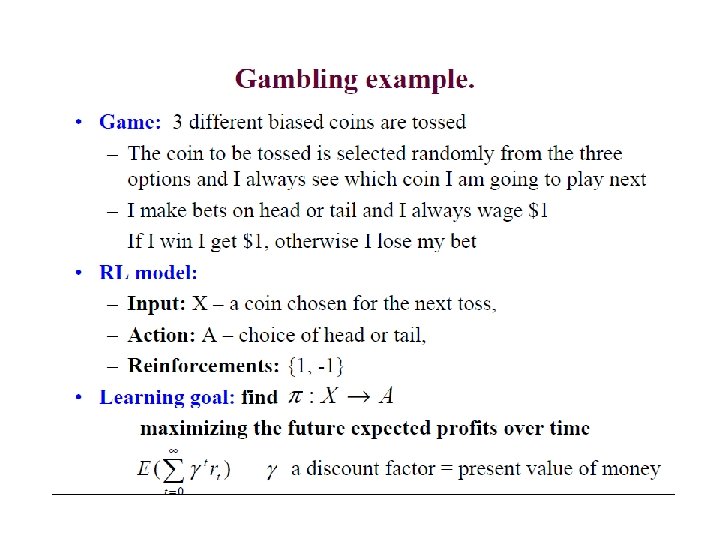
Single State: K-armed Bandit • Among K levers, choose the one that pays best Q(a): value of action a Reward is ra Set Q(a) = ra Choose a* if Q(a*)=maxa Q(a) Rewards stochastic (keep an expected reward): 63
Example: K-armed Bandit • Given $10 to play on a slot machine with 5 levers: – Each play costs $1; each pull of a lever may produce payoff of 0, 1$, 5$, 10$ – Find the optimal policy that pay off the most. • Tradeoff between exploitation and exploration –Exploitation: continue to pull the lever that returns positive – Exploration: try to pull a new one • Deterministic model – The payoff of each lever is fixed, but unknown in advance • Stochastic model – The pay of each lever is uncertainty, with known or unknown probability 64 C. Xu, 2008
K-armed Bandit in General • In deterministic case: Q(a): value of action a Reward of act a is ra Q(a)= ra * if Choose a • Q(a*)=maxa Q(a) 65 • In stochastic model: – Reward is non-deterministic: p(r|a) – Qt(a): estimate of the value of act a at time t • Delta Rule • is learning factor • Qt+1(a) is expected value and should converge to the mean of p(r|a) as t increases C. Xu, 2008
K-Armed Bandit as Simplified RL • Single state (single slot machine) vs Multiple States – p(r|si , aj) : different reward probabilities – Q(Si aj ): value of action aj in state si to be learnt • Action causes state change, in addition to reward • Rewards are not necessarily immediate value – Delayed rewards Start S 2 S 4 S 3 S 8 66 S 5 C. Xu, 2008 S 7 Goal
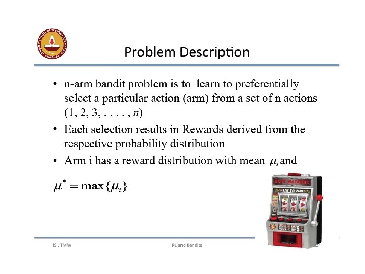
The n-Armed Bandit Problem • Choose repeatedly from one of n actions; each choice is called a play • After each play , you get a reward , where These are unknown action values Distribution of depends only on Objective is to maximize the reward in the long term, e. g. , over 1000 plays To solve the n-armed bandit problem, you must explore a variety of actions and then exploit the best of them. Reinforcement Learning 67
Formalization of RL
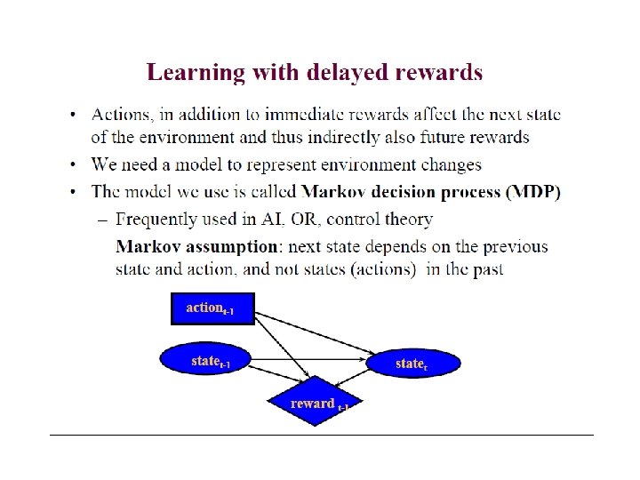
Elements of RL (Markov Decision Processes) • st : State of agent at time t • at: Action taken at time t • In st, action at is taken, clock ticks and reward rt+1 is received and state changes to st+1 • Next state prob: P (st+1 | st , at ) • Reward prob: p (rt+1 | st , at ) • Initial state(s), goal state(s) • Episode (trial) of actions from initial state to goal 69
RL Formalized . . . st at rt +1 st +1 at +1 rt +2 st +2 at +2 rt +3 s t +3 . . . at +3
The Agent Learns a Policy • Reinforcement learning methods specify how the agent changes its policy as a result of experience. • Roughly, the agent’s goal is to get as much reward as it can over the long run.
Getting the Degree of Abstraction Right • Time steps need not refer to fixed intervals of real time. • Actions can be low level (e. g. , voltages to motors), or high level (e. g. , accept a job offer), “mental” (e. g. , shift in focus of attention), etc. • States can be low-level “sensations”, or they can be abstract, symbolic, based on memory, or subjective (e. g. , the state of being “surprised” or “lost”). • Reward computation is in the agent’s environment because the agent cannot change it arbitrarily.
Goals and Rewards • Is a scalar reward signal an adequate notion of a goal? —maybe not, but it is surprisingly flexible. • A goal should specify what we want to achieve, not how we want to achieve it. • A goal must be outside the agent’s direct control— thus outside the agent. • The agent must be able to measure success: – explicitly; – frequently during its lifespan.
Returns Episodic tasks: interaction breaks naturally into episodes, e. g. , plays of a game, trips through a maze. where T is a final time step at which a terminal state is reached, ending an episode.
Returns for Continuing Tasks Continuing tasks: interaction does not have natural episodes. Discounted return:
Policy and Cumulative Reward • Policy, • Value of a policy, • Finite-horizon: • Infinite horizon: 76
The Markov Property • A state should retain all “essential” information, i. e. , it should have the Markov Property:
Markov Decision Processes • If a reinforcement learning task has the Markov Property, it is a Markov Decision Process (MDP). • If state and action sets are finite, it is a finite MDP. • To define a finite MDP, you need to give: – state and action sets – one-step “dynamics” defined by state transition probabilities: – expected rewards:
Value Functions • The value of a state is the expected return starting from that state; depends on the agent’s policy: • The value of taking an action in a state under policy p is the expected return starting from that state, taking that action, and thereafter following p :
Bellman Equation for a Policy p The basic idea: So: Or, without the expectation operator:
Model-Based Learning Environment, P (st+1 | st , at ), p (rt+1 | st , at ), is known There is no need for exploration Can be solved using dynamic programming Solve for Optimal policy 83
Value Iteration 84
Policy Iteration 85
Temporal Difference learning
Temporal Difference Learning • Environment, P (st+1 | st , at ), p (rt+1 | st , at ), is not known; model-free learning • There is need for exploration to sample from P (st+1 | st , at ) and p (rt+1 | st , at ) • Use the reward received in the next time step to update the value of current state (action) • The temporal difference between the value of the current action and the value discounted from the next state 87
Exploration Strategies ε-greedy: With pr ε, choose one action at random uniformly; and choose the best action with pr 1 -ε Probabilistic: Move smoothly from exploration/exploitation. Decrease ε Annealing 88
Deterministic Rewards and Actions Deterministic: single possible reward and next state used as an update rule (backup) Starting at zero, Q values increase, never decrease 89
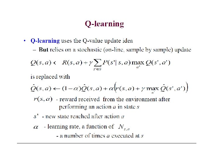
Nondeterministic Rewards and Actions When next states and rewards are nondeterministic (there is an opponent or randomness in the environment), we keep averages (expected values) instead as assignments Q-learning (Watkins and Dayan, 1992): Off-policy vs on-policy (Sarsa) Learning V (TD-learning: Sutton, 1988) 90
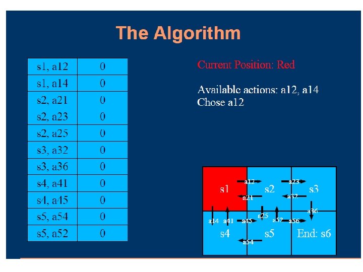
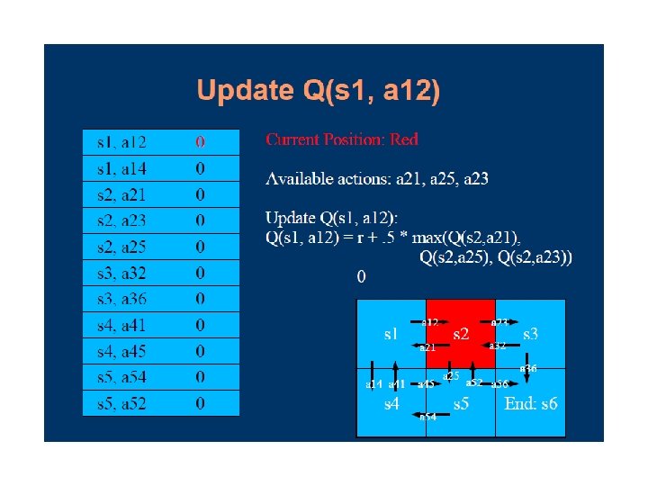
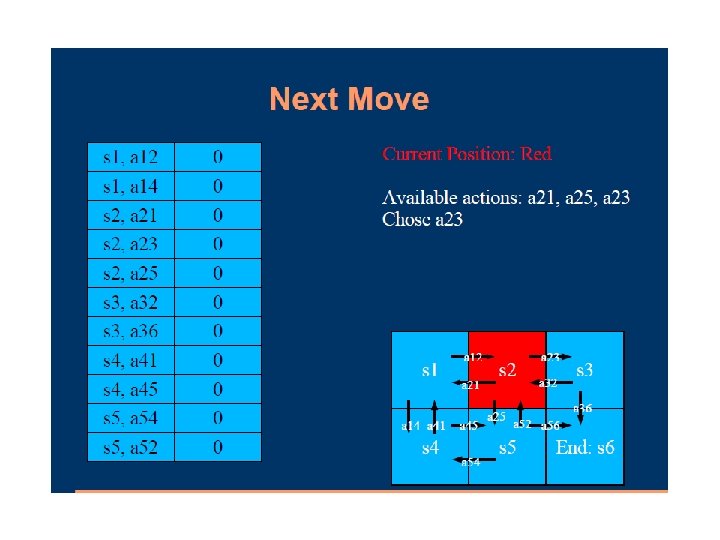
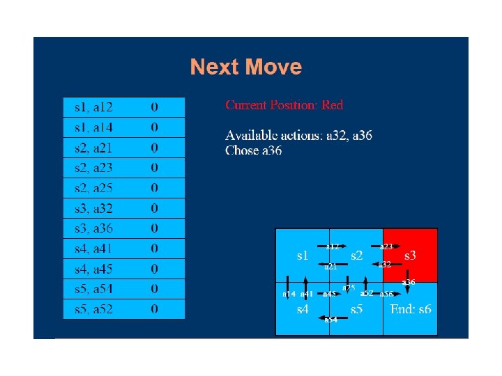
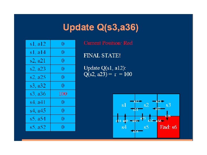
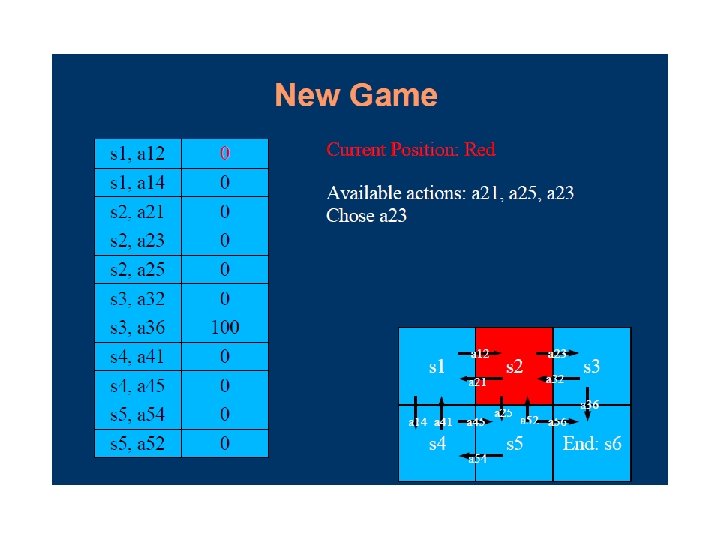
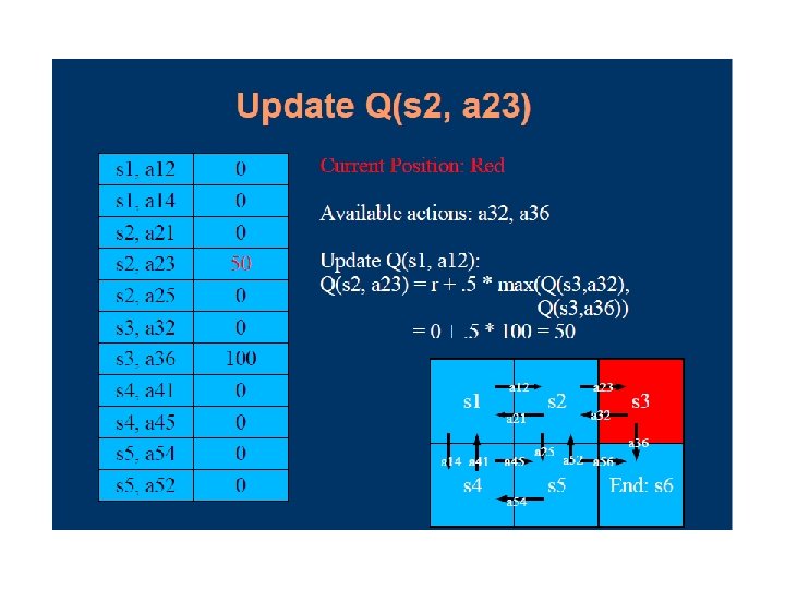
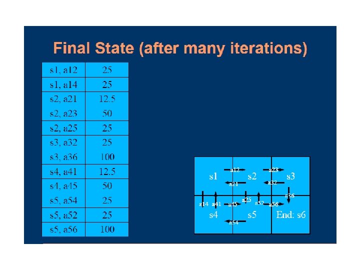
Q Learning
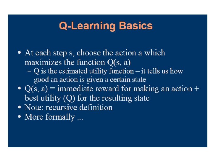
Q-Learning • Q-learning augments value iteration by maintaining an estimated utility value Q(s, a) for every action at every state • The utility of a state U(s), or Q(s), is simply the maximum Q value over all the possible actions at that state • Learns utilities of actions (not states) model -free learning
Selecting an Action • Simply choose action with highest (current) expected utility? • Problem: each action has two effects – yields a reward (or penalty) on current sequence – information is received and used in learning for future sequences stuck in a rut • Trade-off: immediate good for long-term well-being try a shortcut – you might get lost; you might learn a new, quicker route!
Q-learning Lecture Notes for E Alpaydın 2010 Introduction to Machine Learning 2 e © The MIT Press (V 1. 0) 97
Sarsa 109
Partially Observable States • The agent does not know its state but receives an observation which can be used to infer a belief about states • Partially observable MDP 110