Reinforcement Learning for Intelligent Agents Environment Reward Observation

Reinforcement Learning for Intelligent Agents Environment Reward Observation Reasoning Martijn van Otterlo (otterlo@cs. utwente. nl) http: //www. cs. utwente. nl/~otterlo University of Twente SIKS course on “Learning and Reasoning” 21 st May 2007 Action Learning

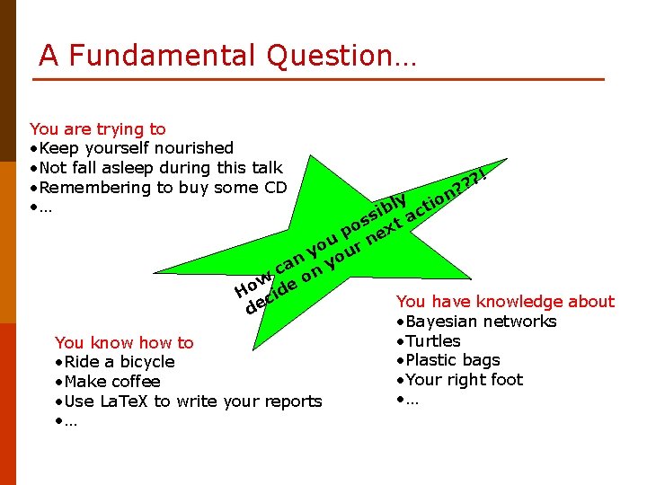
A Fundamental Question… You are trying to • Keep yourself nourished • Not fall asleep during this talk • Remembering to buy some CD • … ? ! ? n? o ti ly b i s t ac s po nex u yo our n ca on y w e o H cid You have knowledge about de • Bayesian networks • Turtles You know how to • Plastic bags • Ride a bicycle • Your right foot • Make coffee • … • Use La. Te. X to write your reports • …

Topics for Today § § § Learning Agents Markov Decision Processes Decision-Theoretic Planning (DTP) Reinforcement Learning (RL) Generalization Some Advanced Topics § § … Partially Observable Problems Hierarchical RL Relational RL I will omit most of the references to the literature. See your reader for links.

Learning Agents § Optimizing agent behavior § § § Programming Planning and Search Learning § RL and DTP as a paradigm; a set of tasks § Features: § § § § Learning from interaction Learning from (numerical) rewards Delayed consequences! Explore-exploit dilemma Goal-directed learning Uncertainty and non-deterministic worlds Rewards (positive) and punishments (negative) Background: psychology (animal and human learning, behaviorism), optimization, control theory (neuro-dynamic programming), operations research, AI/agents, planning/search.

How to learn optimal behavior? § Thorndike’s law of effect (1911): If an action leads to a satisfactory state of affairs, then the tendency of the system to produce that particular action is strengthed or reinforced. Otherwise this tendency is weakened. § Rewards play an important role in reinforcement learning. In fact, it is the only feedback the learner gets and it should be used to optimize action selection.

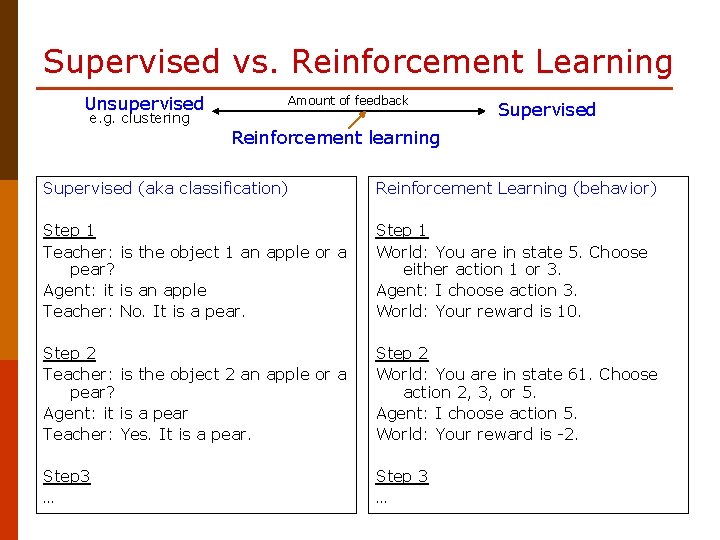
Supervised vs. Reinforcement Learning Unsupervised e. g. clustering Amount of feedback Supervised Reinforcement learning Supervised (aka classification) Reinforcement Learning (behavior) Step 1 Teacher: is the object 1 an apple or a pear? Agent: it is an apple Teacher: No. It is a pear. Step 1 World: You are in state 5. Choose either action 1 or 3. Agent: I choose action 3. World: Your reward is 10. Step 2 Teacher: is the object 2 an apple or a pear? Agent: it is a pear Teacher: Yes. It is a pear. Step 2 World: You are in state 61. Choose action 2, 3, or 5. Agent: I choose action 5. World: Your reward is -2. Step 3 …

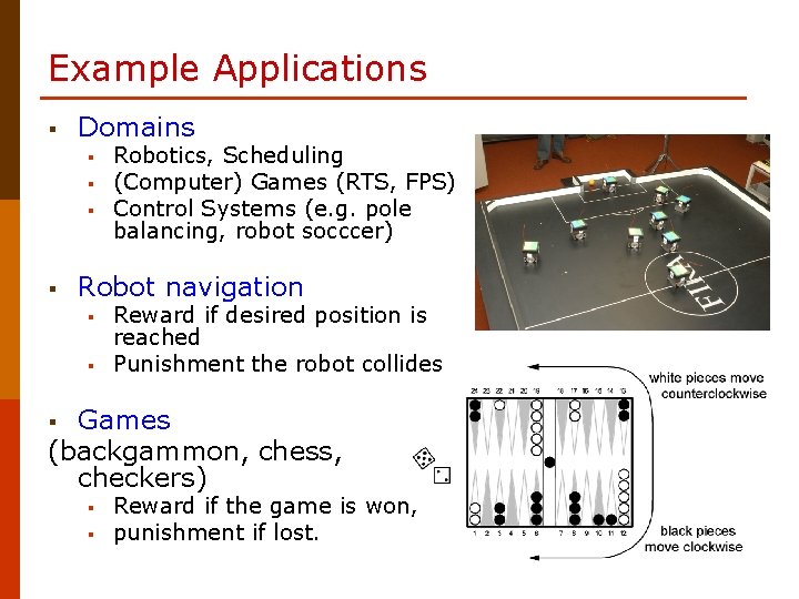
Example Applications § Domains § § Robotics, Scheduling (Computer) Games (RTS, FPS) Control Systems (e. g. pole balancing, robot socccer) Robot navigation § § Reward if desired position is reached Punishment the robot collides Games (backgammon, chess, checkers) § § § Reward if the game is won, punishment if lost.

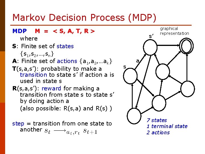
Markov Decision Process (MDP) MDP M = < S, A, T, R > where S: Finite set of states {s 1, s 2, …, sn} A: Finite set of actions {a 1, a 2, …ak} T(s, a, s’): probability to make a transition to state s’ if action a is used in state s R(s, a, s’): reward for making a transition from state s to state s’ by doing action a (also possible: R(s, a) and R(s) ) step = transition from one state to another s’ s graphical representation a 7 states 1 terminal state 2 actions

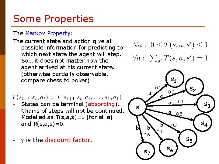
Some Properties The Markov Property: The current state and action give all possible information for predicting to which next state the agent will step. So… it does not matter how the agent arrived at his current state. (otherwise partially observable, compare chess to poker): s 1 a § § States can be terminal (absorbing). Chains of steps will not be continued. Modelled as T(s, a, s)=1 (for all a) and R(s, a, s)=0. is the discount factor. 0. 1 a s b b 0. 6 s 7 b s 2 0. 3 a 0. 1 a 0. 5 s 3 s 4 0. 3 0. 1 s 6 s 5

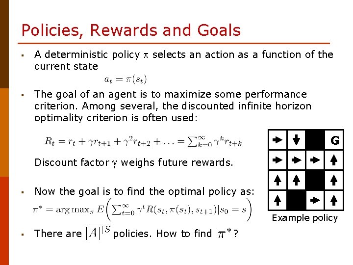
Policies, Rewards and Goals § A deterministic policy selects an action as a function of the current state § The goal of an agent is to maximize some performance criterion. Among several, the discounted infinite horizon optimality criterion is often used: G Discount factor § weighs future rewards. Now the goal is to find the optimal policy as: Example policy § There are policies. How to find ?

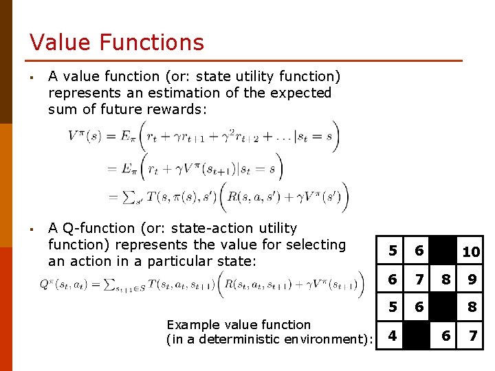
Value Functions § A value function (or: state utility function) represents an estimation of the expected sum of future rewards: § A Q-function (or: state-action utility function) represents the value for selecting an action in a particular state: Example value function (in a deterministic environment): 5 6 6 7 5 6 4 10 8 9 8 6 7

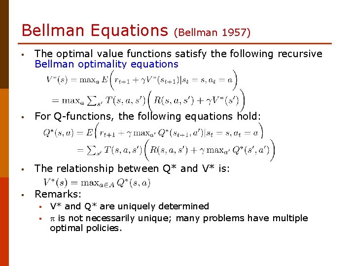
Bellman Equations (Bellman 1957) § The optimal value functions satisfy the following recursive Bellman optimality equations § For Q-functions, the following equations hold: § The relationship between Q* and V* is: § Remarks: § § V* and Q* are uniquely determined is not necessarily unique; many problems have multiple optimal policies.

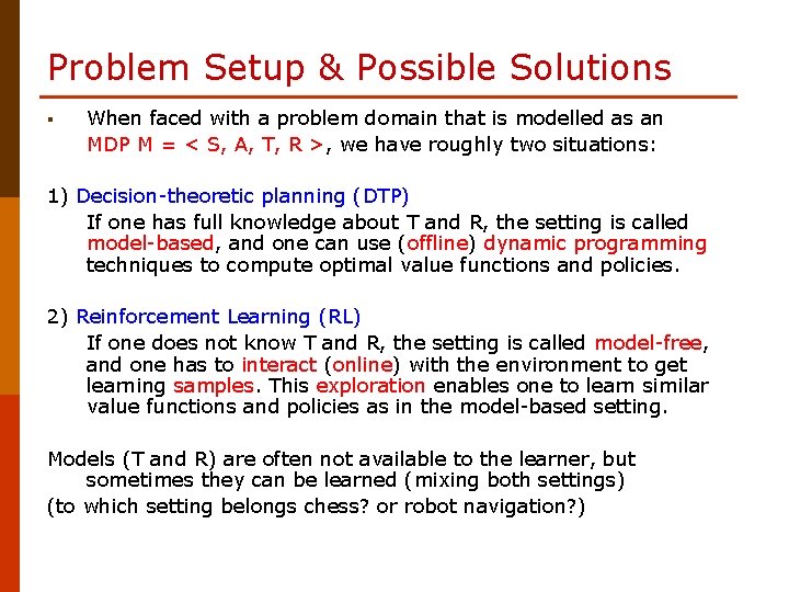
Problem Setup & Possible Solutions § When faced with a problem domain that is modelled as an MDP M = < S, A, T, R >, we have roughly two situations: 1) Decision-theoretic planning (DTP) If one has full knowledge about T and R, the setting is called model-based, and one can use (offline) dynamic programming techniques to compute optimal value functions and policies. 2) Reinforcement Learning (RL) If one does not know T and R, the setting is called model-free, and one has to interact (online) with the environment to get learning samples. This exploration enables one to learn similar value functions and policies as in the model-based setting. Models (T and R) are often not available to the learner, but sometimes they can be learned (mixing both settings) (to which setting belongs chess? or robot navigation? )

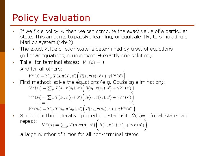
Policy Evaluation § § § If we fix a policy , then we can compute the exact value of a particular state. This amounts to passive learning, or equivalently, to simulating a Markov system (why? ) The exact value of each state is determined by a set of equations (n linear equations, n unknowns exactly one solution) Take, for terminal states: And for all others: § First method: solve the equations (e. g. Gaussian elimination): § Second method: iterative procedure. Start with V(s)=0 for all states and repeat: a large number of times for all non-terminal states

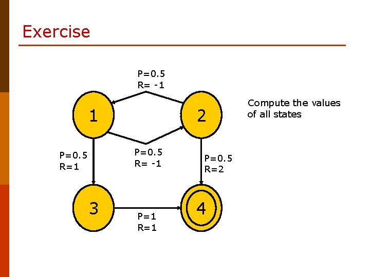
Exercise P=0. 5 R= -1 1 2 P=0. 5 R= -1 P=0. 5 R=1 3 P=1 R=1 P=0. 5 R=2 4 Compute the values of all states

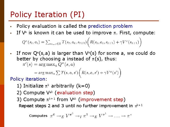
Policy Iteration (PI) § § § Policy evaluation is called the prediction problem If V is known it can be used to improve . First, compute: If now Q (s, a) is larger than V (s) for some a, we could do better by choosing a instead of (s), thus: Policy iteration: 1) Initialize k arbitrarily (k=0) 2) Compute V k (evaluation step) 3) Compute k+1 from V k (improvement step) Repeat steps 2 and 3 until no further improvement in k+1 Computes

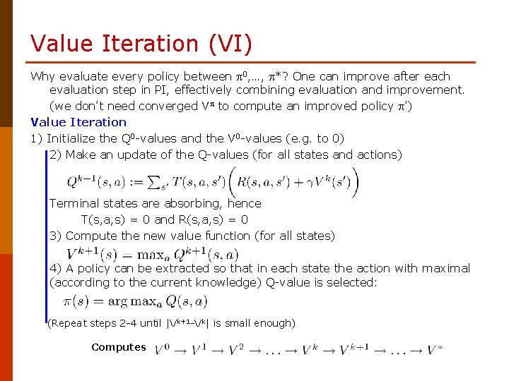
Value Iteration (VI) Why evaluate every policy between 0, …, *? One can improve after each evaluation step in PI, effectively combining evaluation and improvement. (we don’t need converged V to compute an improved policy ’) Value Iteration 1) Initialize the Q 0 -values and the V 0 -values (e. g. to 0) 2) Make an update of the Q-values (for all states and actions) Terminal states are absorbing, hence T(s, a, s) = 0 and R(s, a, s) = 0 3) Compute the new value function (for all states) 4) A policy can be extracted so that in each state the action with maximal (according to the current knowledge) Q-value is selected: (Repeat steps 2 -4 until |Vk+1 -Vk| is small enough) Computes

Some Things about PI and VI § VI turns the Bellman optimality equations into backups, whereas PI separates evaluation and improvement. VI computes a series of approximations of V*, whereas PI computes a series of value functions for distinct intermediate policies. Both kind of setups allow for various extensions. § Both algorithms converge to an optimal value function and policy in the limit, and both have a complexity polynomial in the number of states. § Which one converges faster depends on the problem. In practice, PI needs few iterations, but each iteration involves an expensive evaluation step. § Both VI and PI, and in fact most algorithms that solve MDPs, can be seen as implementing generalized policy iteration (GPI).

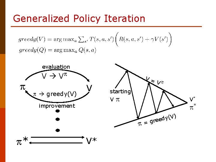
Generalized Policy Iteration evaluation V V greedy(V) V V= V starting V improvement V* * * V* y(V) d e e = gr

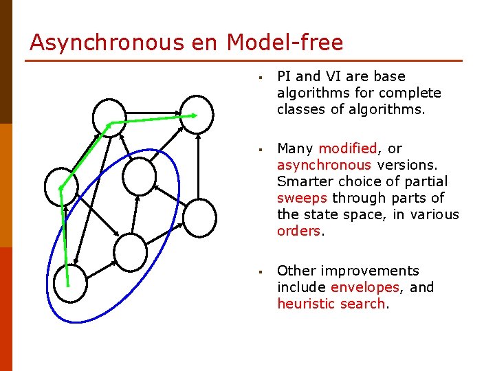
Asynchronous en Model-free § PI and VI are base algorithms for complete classes of algorithms. § Many modified, or asynchronous versions. Smarter choice of partial sweeps through parts of the state space, in various orders. § Other improvements include envelopes, and heuristic search.

Pros and Cons of DTP § Planning § § § DTP § § compute a sequence of actions to reach some goal problem: non-deterministic or probabilistic environments can be used for MDPs, numerical rewards computes reactive policies (instead of plans). advantage: just execute (without costly planning) the optimal action and then follow the policy afterwards. Disadvantages § § One needs the model (T and R) Many states many sweeps over a large space How to deal with continuous states/actions? What about non-Markovian environments?

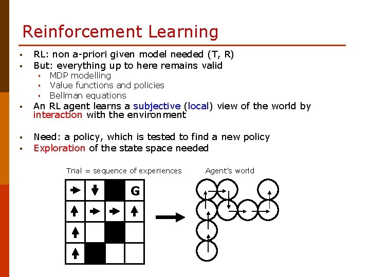
Reinforcement Learning § § RL: non a-priori given model needed (T, R) But: everything up to here remains valid § § § MDP modelling Value functions and policies Bellman equations § An RL agent learns a subjective (local) view of the world by interaction with the environment § Need: a policy, which is tested to find a new policy Exploration of the state space needed § Trial = sequence of experiences G Agent’s world

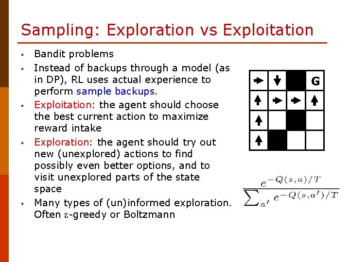
Sampling: Exploration vs Exploitation § § § Bandit problems Instead of backups through a model (as in DP), RL uses actual experience to perform sample backups. Exploitation: the agent should choose the best current action to maximize reward intake Exploration: the agent should try out new (unexplored) actions to find possibly even better options, and to visit unexplored parts of the state space Many types of (un)informed exploration. Often -greedy or Boltzmann G

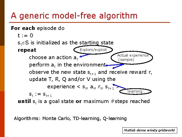
A generic model-free algorithm For each episode do t : = 0 st S is initialized as the starting state Explore/exploit repeat Actual experience choose an action at (sample) perform at in the environment observe the new state st+1 and receive reward rt update T, R, Q and/or V using the experience < st, at, rt, st+1 > learning st : = st+1 until st is a goal state or maximum #steps reached Algorithms: Monte Carlo, TD-learning, Q-learning Matlab demo windy gridworld

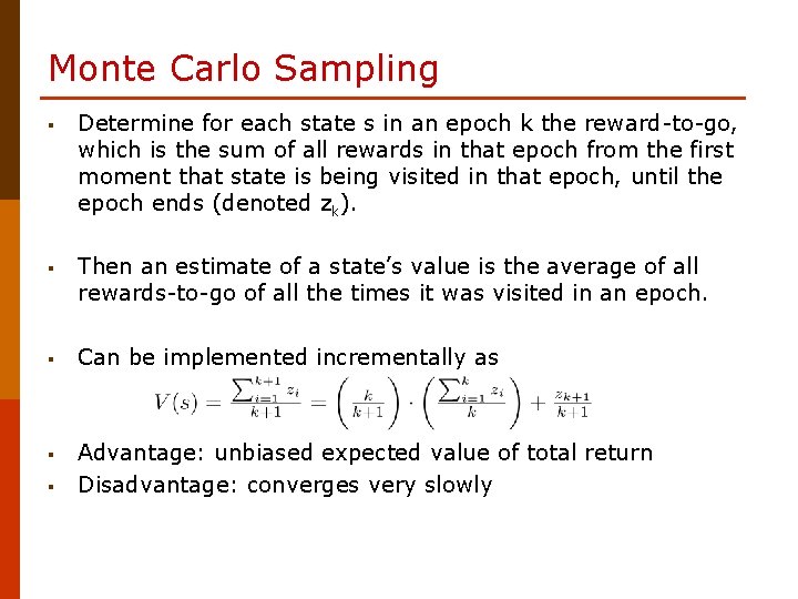
Monte Carlo Sampling § Determine for each state s in an epoch k the reward-to-go, which is the sum of all rewards in that epoch from the first moment that state is being visited in that epoch, until the epoch ends (denoted zk). § Then an estimate of a state’s value is the average of all rewards-to-go of all the times it was visited in an epoch. § Can be implemented incrementally as § Advantage: unbiased expected value of total return Disadvantage: converges very slowly §

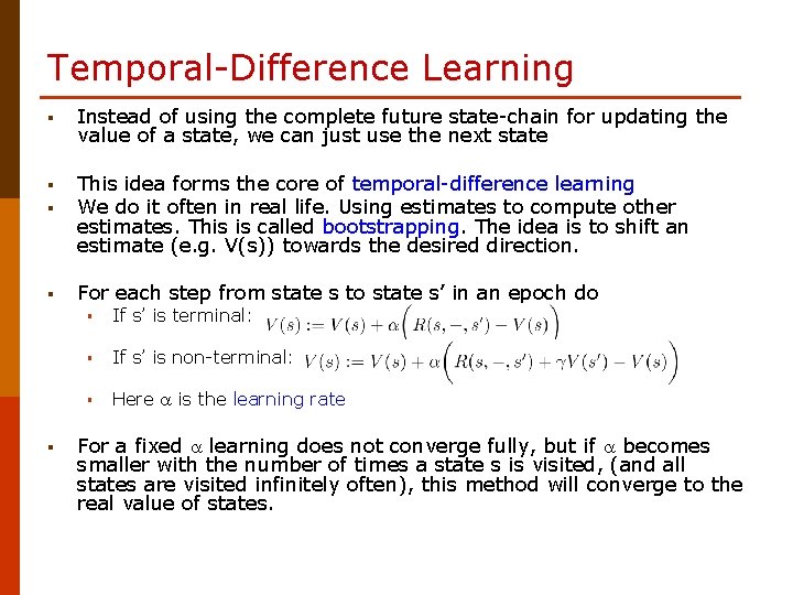
Temporal-Difference Learning § Instead of using the complete future state-chain for updating the value of a state, we can just use the next state § § This idea forms the core of temporal-difference learning We do it often in real life. Using estimates to compute other estimates. This is called bootstrapping. The idea is to shift an estimate (e. g. V(s)) towards the desired direction. § For each step from state s to state s’ in an epoch do § § If s’ is terminal: § If s’ is non-terminal: § Here is the learning rate For a fixed learning does not converge fully, but if becomes smaller with the number of times a state s is visited, (and all states are visited infinitely often), this method will converge to the real value of states.

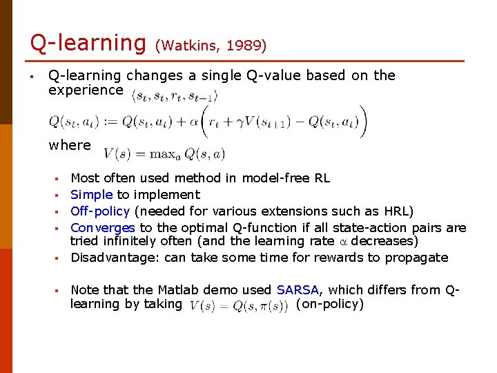
Q-learning § (Watkins, 1989) Q-learning changes a single Q-value based on the experience where § § § Most often used method in model-free RL Simple to implement Off-policy (needed for various extensions such as HRL) Converges to the optimal Q-function if all state-action pairs are tried infinitely often (and the learning rate decreases) Disadvantage: can take some time for rewards to propagate Note that the Matlab demo used SARSA, which differs from Qlearning by taking (on-policy)

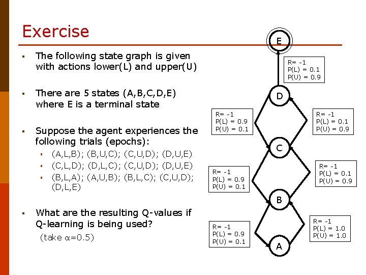
Exercise § The following state graph is given with actions lower(L) and upper(U) § There are 5 states (A, B, C, D, E) where E is a terminal state § Suppose the agent experiences the following trials (epochs): § § § (A, L, B); (B, U, C); (C, U, D); (D, U, E) (C, L, D); (D, L, C); (C, U, D); (D, U, E) (B, L, A); (A, U, B); (B, L, C); (C, U, D); (D, L, E) E R= -1 P(L) = 0. 1 P(U) = 0. 9 D R= -1 P(L) = 0. 9 P(U) = 0. 1 R= -1 P(L) = 0. 1 P(U) = 0. 9 C R= -1 P(L) = 0. 1 P(U) = 0. 9 R= -1 P(L) = 0. 9 P(U) = 0. 1 B § What are the resulting Q-values if Q-learning is being used? (take =0. 5) R= -1 P(L) = 0. 9 P(U) = 0. 1 R= -1 P(L) = 1. 0 P(U) = 1. 0 A

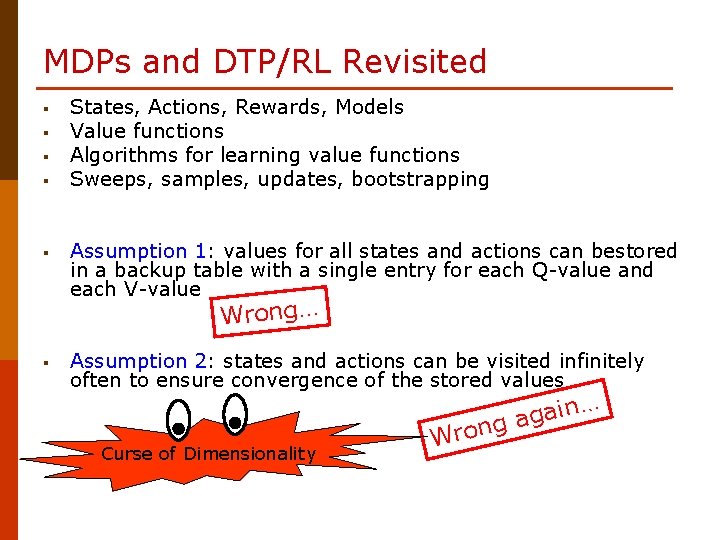
MDPs and DTP/RL Revisited § § § States, Actions, Rewards, Models Value functions Algorithms for learning value functions Sweeps, samples, updates, bootstrapping Assumption 1: values for all states and actions can bestored in a backup table with a single entry for each Q-value and each V-value Wrong… § Assumption 2: states and actions can be visited infinitely often to ensure convergence of the stored values Curse of Dimensionality in… a g Wron

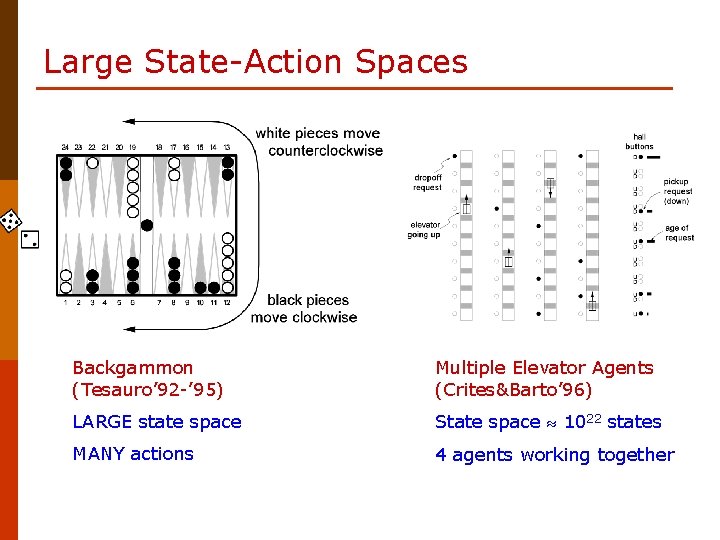
Large State-Action Spaces Backgammon (Tesauro’ 92 -’ 95) Multiple Elevator Agents (Crites&Barto’ 96) LARGE state space State space 1022 states MANY actions 4 agents working together

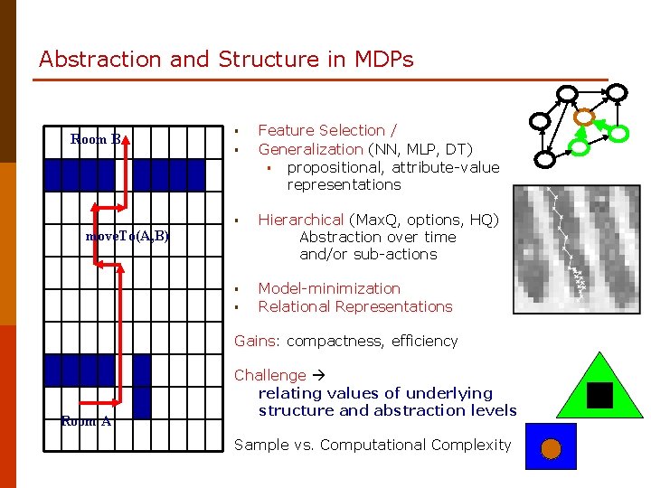
Abstraction and Structure in MDPs Room B § § Feature Selection / Generalization (NN, MLP, DT) § propositional, attribute-value representations § Hierarchical (Max. Q, options, HQ) Abstraction over time and/or sub-actions § Model-minimization Relational Representations move. To(A, B) § Gains: compactness, efficiency Room A Challenge relating values of underlying structure and abstraction levels Sample vs. Computational Complexity

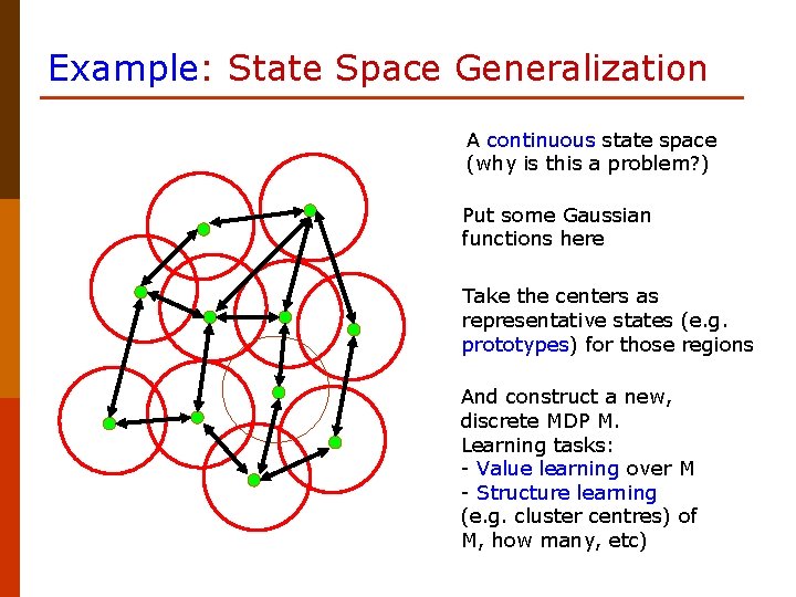
Example: State Space Generalization A continuous state space (why is this a problem? ) Put some Gaussian functions here Take the centers as representative states (e. g. prototypes) for those regions And construct a new, discrete MDP M. Learning tasks: - Value learning over M - Structure learning (e. g. cluster centres) of M, how many, etc)

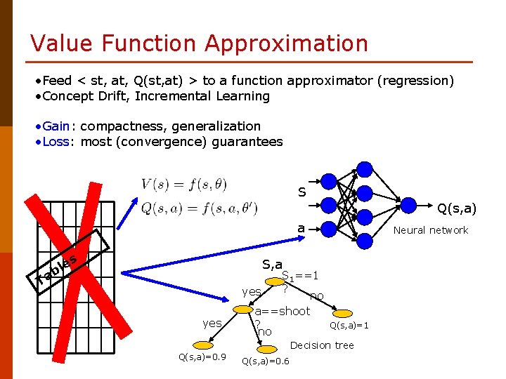
Value Function Approximation • Feed < st, at, Q(st, at) > to a function approximator (regression) • Concept Drift, Incremental Learning • Gain: compactness, generalization • Loss: most (convergence) guarantees S Q(s, a) a T es l ab Neural network S, a yes S 1==1 ? yes no a==shoot ? no Q(s, a)=1 Decision tree Q(s, a)=0. 9 Q(s, a)=0. 6

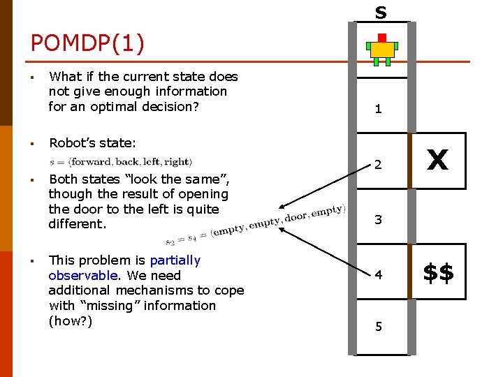
S POMDP(1) § § What if the current state does not give enough information for an optimal decision? 1 Robot’s state: Both states “look the same”, though the result of opening the door to the left is quite different. This problem is partially observable. We need additional mechanisms to cope with “missing” information (how? ) 2 X 3 4 5 $$

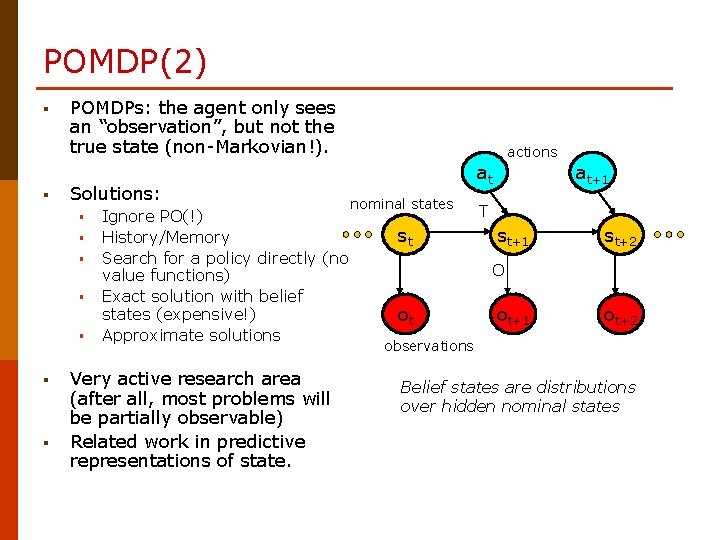
POMDP(2) § § POMDPs: the agent only sees an “observation”, but not the true state (non-Markovian!). Solutions: § § § § Ignore PO(!) History/Memory Search for a policy directly (no value functions) Exact solution with belief states (expensive!) Approximate solutions Very active research area (after all, most problems will be partially observable) Related work in predictive representations of state. actions at nominal states st at+1 T st+1 st+2 O ot ot+1 ot+2 observations Belief states are distributions over hidden nominal states

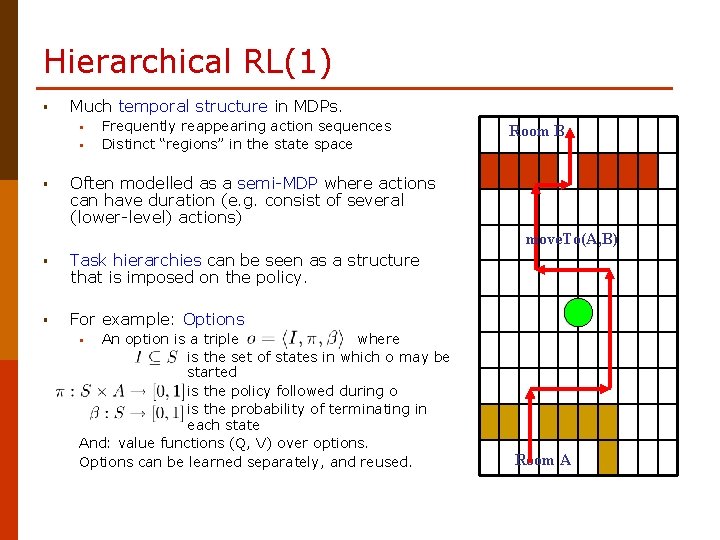
Hierarchical RL(1) § Much temporal structure in MDPs. § § § Frequently reappearing action sequences Distinct “regions” in the state space Room B Often modelled as a semi-MDP where actions can have duration (e. g. consist of several (lower-level) actions) move. To(A, B) § Task hierarchies can be seen as a structure that is imposed on the policy. § For example: Options An option is a triple where is the set of states in which o may be started is the policy followed during o is the probability of terminating in each state And: value functions (Q, V) over options. Options can be learned separately, and reused. § Room A

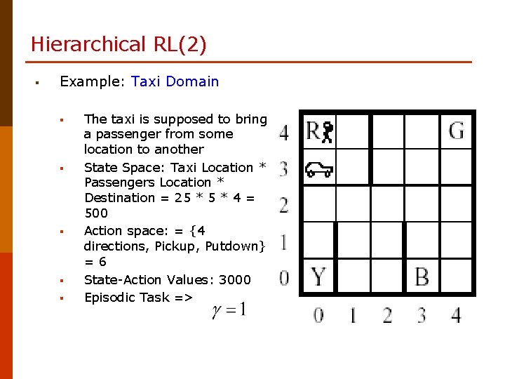
Hierarchical RL(2) § Example: Taxi Domain § § § The taxi is supposed to bring a passenger from some location to another State Space: Taxi Location * Passengers Location * Destination = 25 * 4 = 500 Action space: = {4 directions, Pickup, Putdown} =6 State-Action Values: 3000 Episodic Task =>

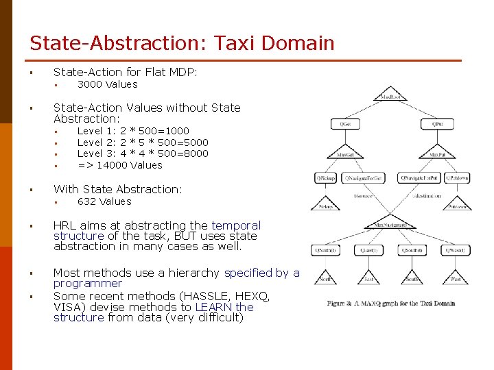
State-Abstraction: Taxi Domain § State-Action for Flat MDP: § § State-Action Values without State Abstraction: § § § 3000 Values Level 1: 2 * 500=1000 Level 2: 2 * 500=5000 Level 3: 4 * 500=8000 => 14000 Values With State Abstraction: § 632 Values § HRL aims at abstracting the temporal structure of the task, BUT uses state abstraction in many cases as well. § Most methods use a hierarchy specified by a programmer Some recent methods (HASSLE, HEXQ, VISA) devise methods to LEARN the structure from data (very difficult) §

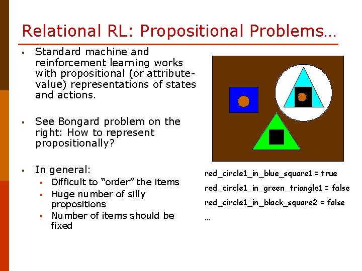
Relational RL: Propositional Problems… § Standard machine and reinforcement learning works with propositional (or attributevalue) representations of states and actions. § See Bongard problem on the right: How to represent propositionally? § In general: § § § Difficult to “order” the items Huge number of silly propositions Number of items should be fixed red_circle 1_in_blue_square 1 = true red_circle 1_in_green_triangle 1 = false red_circle 1_in_black_square 2 = false …

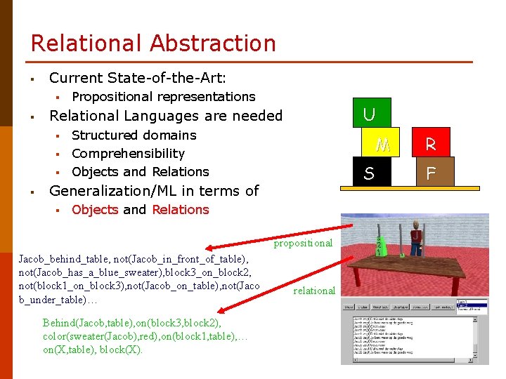
Relational Abstraction § Current State-of-the-Art: § § U Relational Languages are needed § § Propositional representations Structured domains Comprehensibility Objects and Relations M S Generalization/ML in terms of § Objects and Relations propositional Jacob_behind_table, not(Jacob_in_front_of_table), not(Jacob_has_a_blue_sweater), block 3_on_block 2, not(block 1_on_block 3), not(Jacob_on_table), not(Jaco b_under_table)… Behind(Jacob, table), on(block 3, block 2), color(sweater(Jacob), red), on(block 1, table), … on(X, table), block(X). relational R F

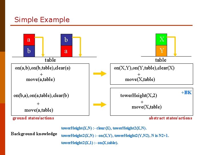
Simple Example a b X b a Y table on(a, b), on(b, table), clear(a) + move(a, table) on(X, Y), on(Y, table), clear(X) + move(X, table) on(b, a), on(a, table), clear(b) + move(a, table) tower. Height(X, 2) + move(X, table) ground states/actions +BK abstract states/actions tower. Height(X, N) : - clear(X), tower. Height 2(X, N). Background knowledge tower. Height 2(X, N) : - on(X, Y), tower. Height 2(Y, N 2), N is N 2+1. tower. Height 2(X, 1) : - on(X, table).

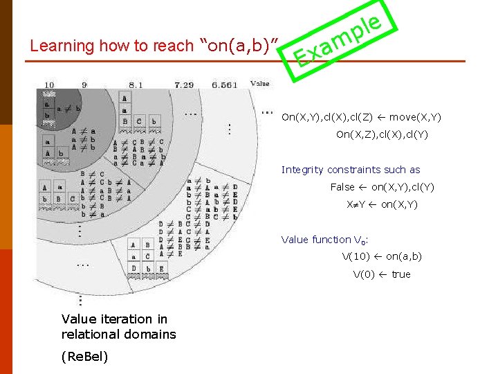
Learning how to reach “on(a, b)” le p m a x E On(X, Y), cl(X), cl(Z) move(X, Y) On(X, Z), cl(X), cl(Y) Integrity constraints such as False on(X, Y), cl(Y) X Y on(X, Y) Value function V 0: V(10) on(a, b) V(0) true Value iteration in relational domains (Re. Bel)

Wrap-up(1): Summary § Reinforcement learning and decision-theoretic planning aim at learning behavior, based on the concepts of states, actions and rewards. Delayed effects and the need for exploration are important. § Many methods exit for learning value functions (GPI!). There’s reasonable understanding how to do it, for both model-based and model-free settings. Theory is still developing, relating RL to classification learning. § Function approximation, abstraction and generalization make the learning problem more compact, and aim at generalization over domain structures. § Relational RL upgrades the whole framework by using a higher-order language and aim at higher-order (cognitive) notions (objects!). § Various combinations of spatial and temporal abstraction, and various forms of knowledge representation are being investigated

Wrap-up(2): We did not have time for: § § § § Efficient exploration schemes Eligibility traces Complexity aspects (computational, sample) Continuous models Theory (convergence, optimality, speed) Applications Policy search methods (search, evolution, gradients) Multi-agent learning Game-theoretic learning Predictive representations Connections with planning Connections with cognitive architectures General place of RL within AI … (many more…)