Regression on Time Series Data Part I Dynamics

Regression on Time Series Data - Part I Dynamics of Residuals

Forecasting Using Regression 1. Watch for Spurious Regression 2. Check Stationarity of Residuals for Stability of the Relationship – Cointegration 3. Learn Modeling Techniques for Reducing Residuals to WN 4. Aware of Translating The Forecasting Problem to That of Independent Variables

Integrated Process • Integrated Process I(1): (1 - L)Yt = ARMA(p, q)t • Key Model (Hypothesis) for Macroeconomic Variables • Uncertainty of the Long Run Path

Spurious Regression • Two I(1) variables could exhibit significant correlation, without an underlying relationship.

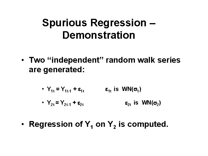
Spurious Regression – Demonstration • Two “independent” random walk series are generated: • Y 1 t = Y 1 t-1 + e 1 t • Y 2 t = Y 2 t-1 + e 2 t e 1 t is WN(s 1) e 2 t is WN(s 2) • Regression of Y 1 on Y 2 is computed.

Key Reminders • The regression must make economic “sense” • Check the residual if “stationary”

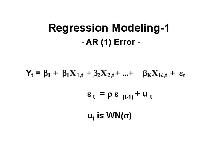
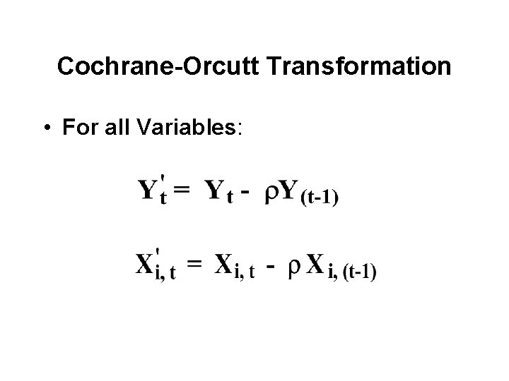
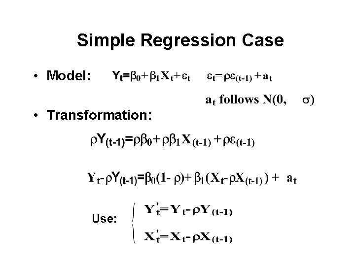
Regression Modeling-1 - AR (1) Error - et =re (t-1) + ut is WN(s) ut

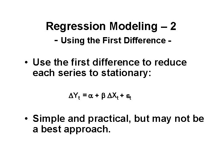
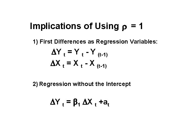
Regression Modeling – 2 - Using the First Difference • Use the first difference to reduce each series to stationary: DYt = a + b DXt + et • Simple and practical, but may not be a best approach.

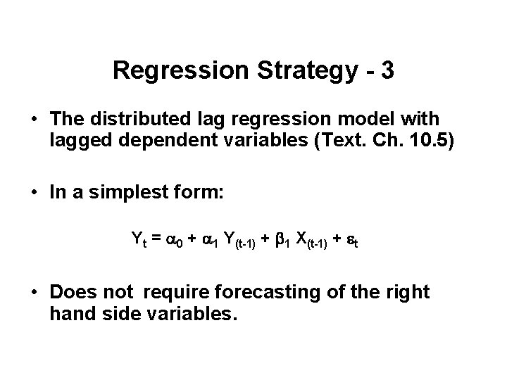
Regression Strategy - 3 • The distributed lag regression model with lagged dependent variables (Text. Ch. 10. 5) • In a simplest form: Yt = a 0 + a 1 Y(t-1) + b 1 X(t-1) + et • Does not require forecasting of the right hand side variables.

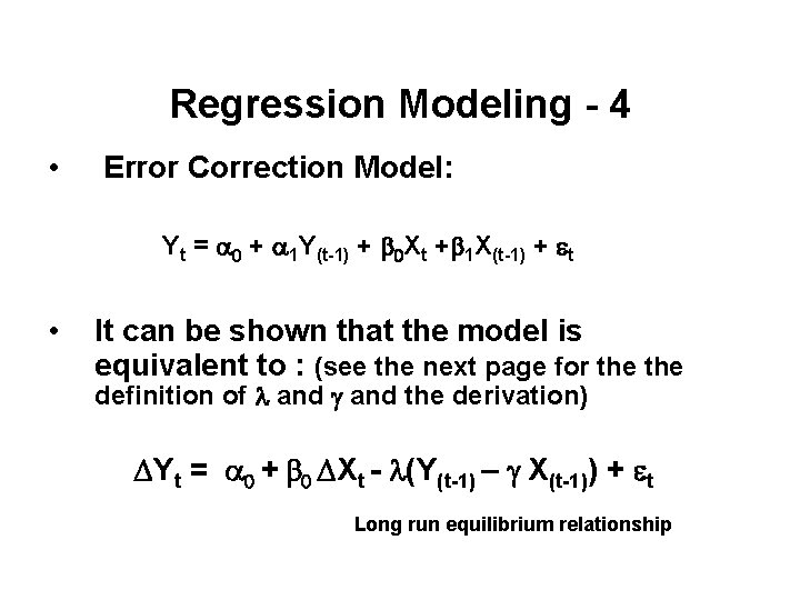
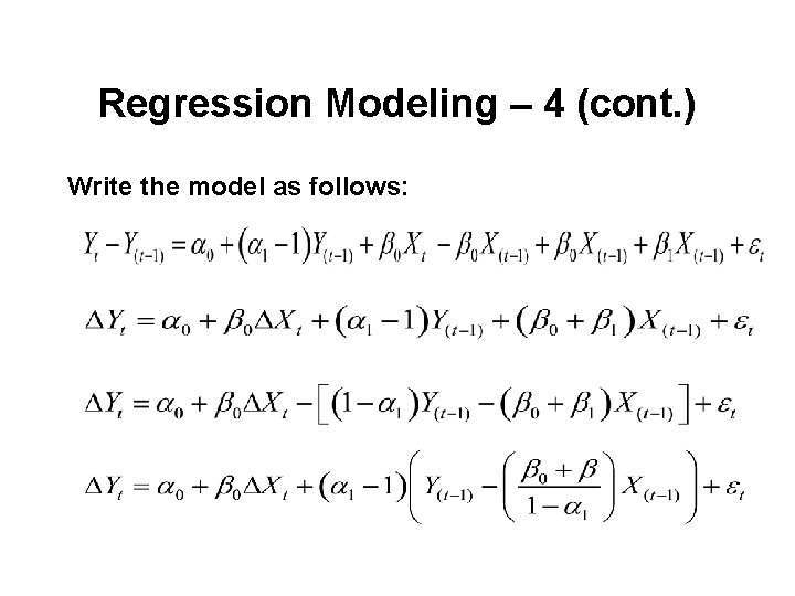
Regression Modeling - 4 • Error Correction Model: Yt = a 0 + a 1 Y(t-1) + b 0 Xt +b 1 X(t-1) + et • It can be shown that the model is equivalent to : (see the next page for the definition of l and g and the derivation) DYt = a 0 + b 0 DXt - l(Y(t-1) – g X(t-1)) + et Long run equilibrium relationship

Regression Modeling – 4 (cont. ) Write the model as follows:

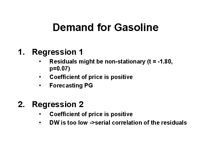
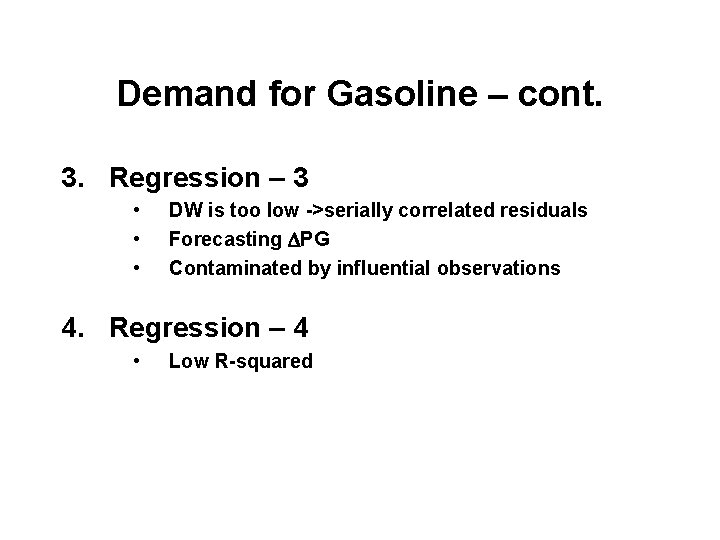
Demand for Gasoline 1. Regression 1 • • • Residuals might be non-stationary (t = -1. 80, p=0. 07) Coefficient of price is positive Forecasting PG 2. Regression 2 • • Coefficient of price is positive DW is too low ->serial correlation of the residuals

Demand for Gasoline – cont. 3. Regression – 3 • • • DW is too low ->serially correlated residuals Forecasting DPG Contaminated by influential observations 4. Regression – 4 • Low R-squared

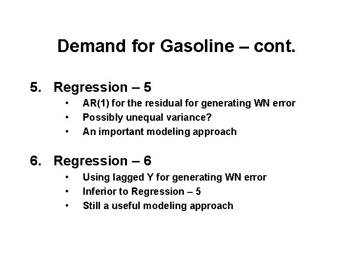
Demand for Gasoline – cont. 5. Regression – 5 • • • AR(1) for the residual for generating WN error Possibly unequal variance? An important modeling approach 6. Regression – 6 • • • Using lagged Y for generating WN error Inferior to Regression – 5 Still a useful modeling approach

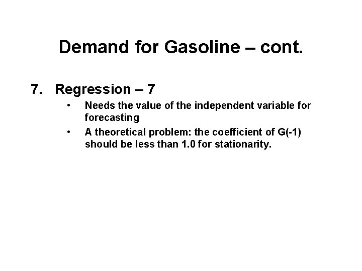
Demand for Gasoline – cont. 7. Regression – 7 • • Needs the value of the independent variable forecasting A theoretical problem: the coefficient of G(-1) should be less than 1. 0 for stationarity.

Appendix: AR(1) Error

Cochrane-Orcutt Transformation • For all Variables:

Simple Regression Case • Model: • Transformation: Use:

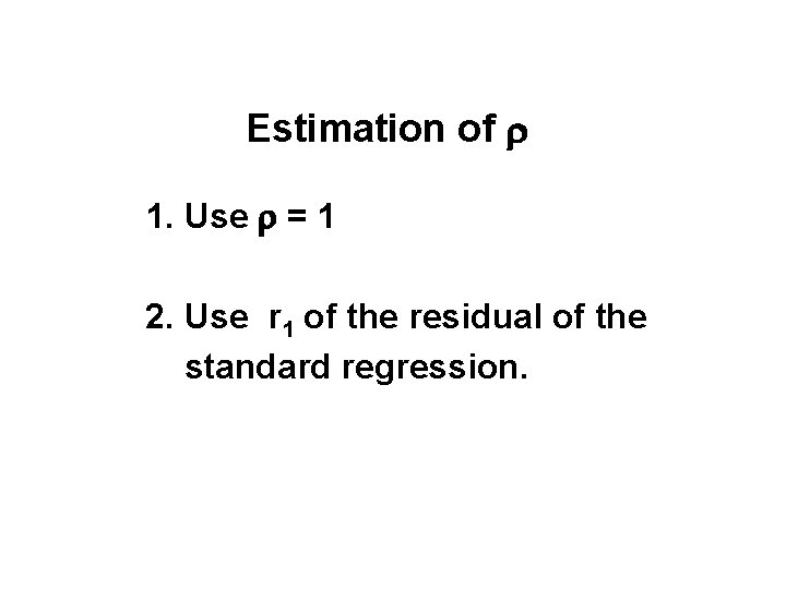
Estimation of r 1. Use r = 1 2. Use r 1 of the residual of the standard regression.

Implications of Using r = 1 1) First Differences as Regression Variables: DY t = Y t - Y (t-1) DX t = X t - X (t-1) 2) Regression without the Intercept DY t = b 1 DX t +at