Regression Models Introduction In regression models there are

Regression Models - Introduction • In regression models there are two types of variables that are studied: Ø A dependent variable, Y, also called response variable. It is modeled as random. Ø An independent variable, X, also called predictor variable or explanatory variable. It is sometimes modeled as random and sometimes it has fixed value for each observation. • In regression models we are fitting a statistical model to data. • We generally use regression to be able to predict the value of one variable given the value of others. STA 261 week 13 1

Simple Linear Regression - Introduction • Simple linear regression studies the relationship between a quantitative response variable Y, and a single explanatory variable X. • Idea of statistical model: Actual observed value of Y = … • Box (a well know statistician) claim: “All models are wrong, some are useful”. ‘Useful’ means that they describe the data well and can be used for predictions and inferences. • Recall: parameters are constants in a statistical model which we usually don’t know but will use data to estimate. STA 261 week 13 2

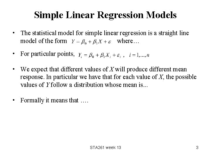
Simple Linear Regression Models • The statistical model for simple linear regression is a straight line model of the form where… • For particular points, • We expect that different values of X will produce different mean response. In particular we have that for each value of X, the possible values of Y follow a distribution whose mean is. . . • Formally it means that …. STA 261 week 13 3

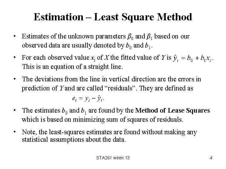
Estimation – Least Square Method • Estimates of the unknown parameters β 0 and β 1 based on our observed data are usually denoted by b 0 and b 1. • For each observed value xi of X the fitted value of Y is This is an equation of a straight line. • The deviations from the line in vertical direction are the errors in prediction of Y and are called “residuals”. They are defined as • The estimates b 0 and b 1 are found by the Method of Lease Squares which is based on minimizing sum of squares of residuals. • Note, the least-squares estimates are found without making any statistical assumptions about the data. STA 261 week 13 4

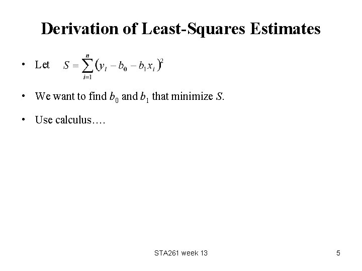
Derivation of Least-Squares Estimates • Let • We want to find b 0 and b 1 that minimize S. • Use calculus…. STA 261 week 13 5

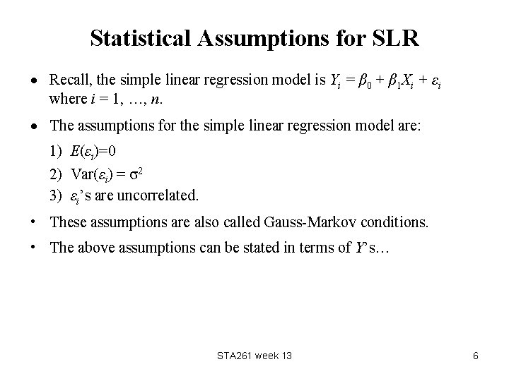
Statistical Assumptions for SLR Recall, the simple linear regression model is Yi = β 0 + β 1 Xi + εi where i = 1, …, n. The assumptions for the simple linear regression model are: 1) E(εi)=0 2) Var(εi) = σ2 3) εi’s are uncorrelated. • These assumptions are also called Gauss-Markov conditions. • The above assumptions can be stated in terms of Y’s… STA 261 week 13 6

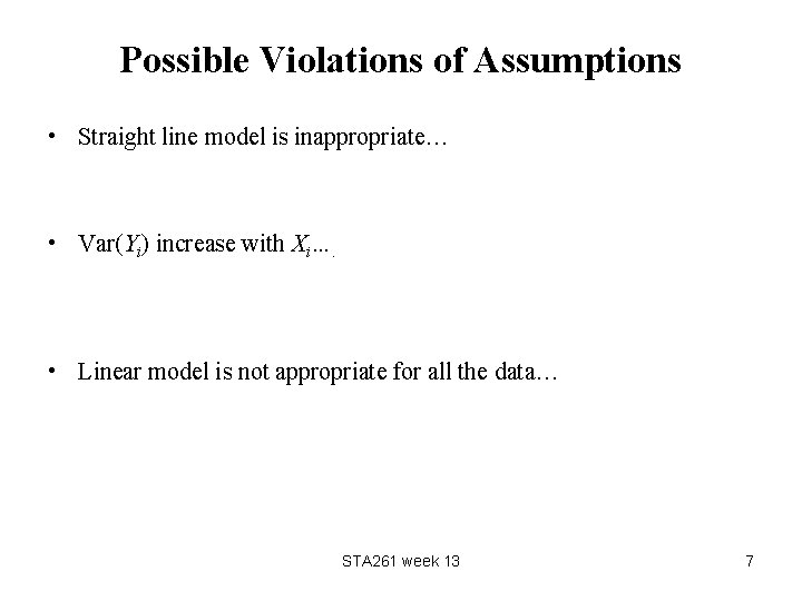
Possible Violations of Assumptions • Straight line model is inappropriate… • Var(Yi) increase with Xi…. • Linear model is not appropriate for all the data… STA 261 week 13 7

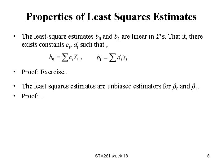
Properties of Least Squares Estimates • The least-square estimates b 0 and b 1 are linear in Y’s. That it, there exists constants ci, di such that , • Proof: Exercise. . • The least squares estimates are unbiased estimators for β 0 and β 1. • Proof: … STA 261 week 13 8

Gauss-Markov Theorem • The least-squares estimates are BLUE (Best Linear, Unbiased Estimators). • Of all the possible linear, unbiased estimators of β 0 and β 1 the least squares estimates have the smallest variance. • The variance of the least-squares estimates is… STA 261 week 13 9

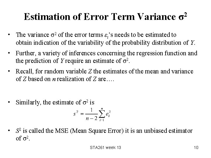
Estimation of Error Term Variance σ2 • The variance σ2 of the error terms εi’s needs to be estimated to obtain indication of the variability of the probability distribution of Y. • Further, a variety of inferences concerning the regression function and the prediction of Y require an estimate of σ2. • Recall, for random variable Z the estimates of the mean and variance of Z based on n realization of Z are…. • Similarly, the estimate of σ2 is • S 2 is called the MSE (Mean Square Error) it is an unbiased estimator of σ2. STA 261 week 13 10

Normal Error Regression Model • In order to make inference we need one more assumption about εi’s. • We assume that εi’s have a Normal distribution, that is εi ~ N(0, σ2). • The Normality assumption implies that the errors εi’s are independent (since they are uncorrelated). • Under the Normality assumption of the errors, the least squares estimates of β 0 and β 1 are equivalent to their maximum likelihood estimators. • This results in additional nice properties of MLE’s: they are consistent, sufficient and MVUE. STA 261 week 13 11

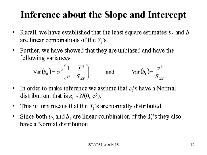
Inference about the Slope and Intercept • Recall, we have established that the least square estimates b 0 and b 1 are linear combinations of the Yi’s. • Further, we have showed that they are unbiased and have the following variances • In order to make inference we assume that εi’s have a Normal distribution, that is εi ~ N(0, σ2). • This in turn means that the Yi’s are normally distributed. • Since both b 0 and b 1 are linear combination of the Yi’s they also have a Normal distribution. STA 261 week 13 12

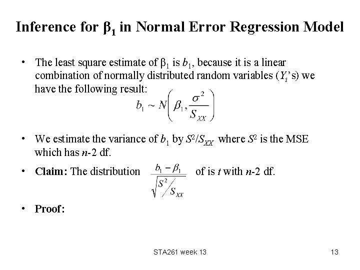
Inference for β 1 in Normal Error Regression Model • The least square estimate of β 1 is b 1, because it is a linear combination of normally distributed random variables (Yi’s) we have the following result: • We estimate the variance of b 1 by S 2/SXX where S 2 is the MSE which has n-2 df. • Claim: The distribution of is t with n-2 df. • Proof: STA 261 week 13 13

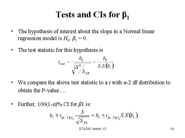
Tests and CIs for β 1 • The hypothesis of interest about the slope in a Normal linear regression model is H 0: β 1 = 0. • The test statistic for this hypothesis is • We compare the above test statistic to a t with n-2 df distribution to obtain the P-value…. • Further, 100(1 -α)% CI for β 1 is: STA 261 week 13 14

Important Comment • Similar results can be obtained about the intercept in a Normal linear regression model. • However, in many cases the intercept does not have any practical meaning and therefore it is not necessary to make inference about it. STA 261 week 13 15