Regression making predictions Correlation vs Regression l Corr

Regression making predictions

Correlation vs. Regression l Corr. l Association l Two variables l Both free to vary l Single coefficient Reg. Prediction X (IV) & Y (DV) X fixed, Y free Predicted values, Residuals, Strength of model statistics

Correlation vs. Regression l Corr. l Descriptive Reg. Inferential l Regression bridges the gap between descriptive and inferential statistics. l It is related to correlation, but is also used to test hypotheses.

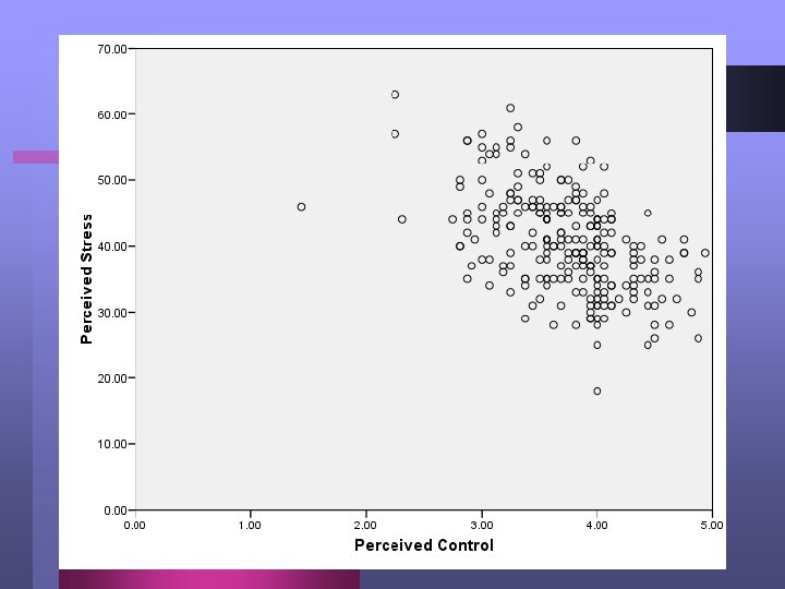
Conceptual Introduction l Linear regression gives us an equation. l The equation describes a line that is the “line of best fit. ” It is the line that best describes the relationship between variables. l Think about shooting an arrow through the scatterplot, so that the arrow passes as close to all the points as possible.

Conceptual Introduction l The “line of best fit”, or the arrow that passes through the scatterplot closest to the points, shows us where our predicted Y values are for given values of X.

Conceptual Introduction l The line is like taking a running mean, or the average of Y for each value of X, and then smoothing it out to make a straight line. l In a sense, our best prediction of Y for a given value of X, is the mean of all the Y values that have the particular value of X in question.

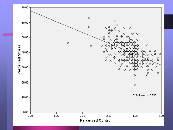
Conceptual Introduction l Remember from algebra, that we describe a line with this equation: l Y = mx + b l In statistics we say: l Y = b 0 + b 1 x 1 + e l Ypred = b 0 + b 1 x 1 where: b 0 = Y intercept b 1 = Slope

Perceived Stress = 67. 651 - 7. 238(Perceived Control) + e Predicted Perceived Stress = 67. 651 - 7. 238(Perceived Control)