Regression Linear regression involves finding the equation of

Regression Linear regression involves finding the equation of the line of best fit on a scatter graph. The equation obtained can then be used to make an estimate of one variable given the value of the other variable. There are two cases to consider, depending upon whether: 1. We wish to find a value of y given a value for x, or 2. We want to estimate x given y. S 1 deals with the first situation.

Regression Linear regression involves finding the equation of the line of best fit on a scatter graph. The equation obtained can then be used to make an estimate of one variable given the value of the other variable. There are two cases to consider, depending upon whether: 1. We wish to find a value of y given a value for x, 2. We want to estimate x given y. S 1 deals with the first situation.

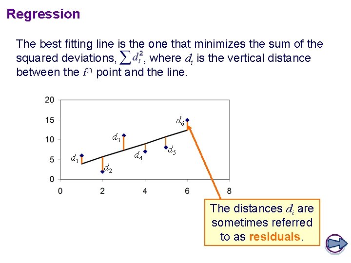
Regression The best fitting line is the one that minimizes the sum of the squared deviations, , where di is the vertical distance between the ith point and the line. d 6 d 3 d 1 d 4 d 5 d 2 The distances di are sometimes referred to as residuals.

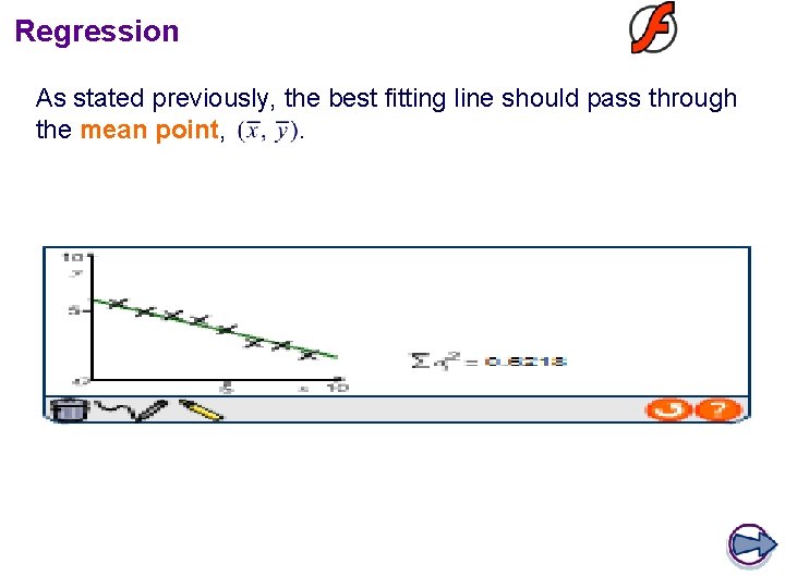
Regression As stated previously, the best fitting line should pass through the mean point, .

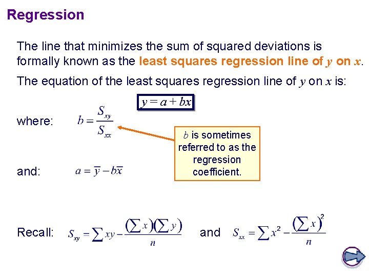
Regression The line that minimizes the sum of squared deviations is formally known as the least squares regression line of y on x. The equation of the least squares regression line of y on x is: y = a + bx where: and: Recall: b is sometimes referred to as the regression coefficient. and

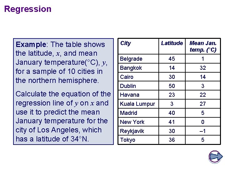
Regression Example: The table shows the latitude, x, and mean January temperature(°C), y, for a sample of 10 cities in the northern hemisphere. City Latitude Mean Jan. temp. (°C) Belgrade 45 1 Bangkok 14 32 Cairo 30 14 Dublin 50 3 Calculate the equation of the regression line of y on x and use it to predict the mean January temperature for the city of Los Angeles, which has a latitude of 34°N. Havana 23 22 Kuala Lumpur 3 27 Madrid 40 5 New York 41 0 Reykjavik 30 – 1 Tokyo 36 5

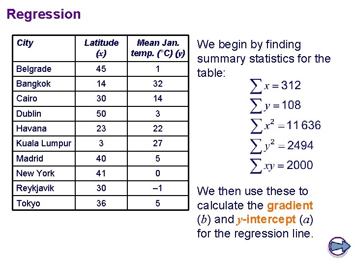
Regression City Latitude (x) Mean Jan. temp. (°C) (y) Belgrade 45 1 Bangkok 14 32 Cairo 30 14 Dublin 50 3 Havana 23 22 Kuala Lumpur 3 27 Madrid 40 5 New York 41 0 Reykjavik 30 – 1 Tokyo 36 5 We begin by finding summary statistics for the table: We then use these to calculate the gradient (b) and y-intercept (a) for the regression line.

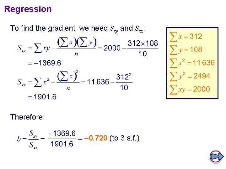
Regression To find the gradient, we need Sxy and Sxx: Therefore: – 0. 720 (to 3 s. f. )

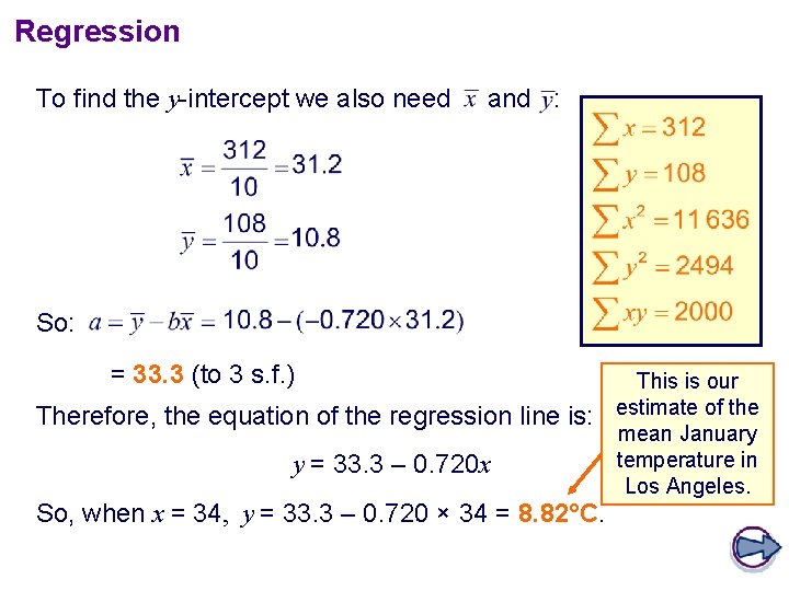
Regression To find the y-intercept we also need and : So: = 33. 3 (to 3 s. f. ) Therefore, the equation of the regression line is: y = 33. 3 – 0. 720 x So, when x = 34, y = 33. 3 – 0. 720 × 34 = 8. 82°C. This is our estimate of the mean January temperature in Los Angeles.

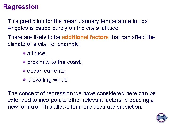
Regression This prediction for the mean January temperature in Los Angeles is based purely on the city’s latitude. There are likely to be additional factors that can affect the climate of a city, for example: altitude; proximity to the coast; ocean currents; prevailing winds. The concept of regression we have considered here can be extended to incorporate other relevant factors, producing a new formula. This allows for more accurate prediction.

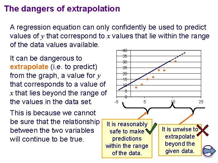
The dangers of extrapolation A regression equation can only confidently be used to predict values of y that correspond to x values that lie within the range of the data values available. It can be dangerous to extrapolate (i. e. to predict) from the graph, a value for y that corresponds to a value of x that lies beyond the range of the values in the data set. 40 35 30 25 20 15 10 5 0 -5 5 This is because we cannot be sure that the relationship It is reasonably between the two variables safe to make predictions will continue to be true. within the range of the data. 15 It is unwise to extrapolate beyond the given data. 25

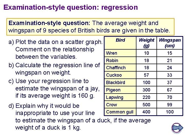
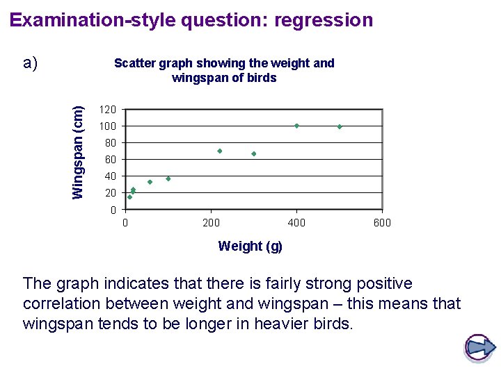
Examination-style question: regression Examination-style question: The average weight and wingspan of 9 species of British birds are given in the table. a) Plot the data on a scatter graph. Comment on the relationship between the variables. b) Calculate the regression line of wingspan on weight. c) Use your regression line to estimate the wingspan of a jay, if its average weight is 160 g. Bird Weight Wingspan (g) (cm) Wren 10 15 Robin 18 21 Chaffinch 18 24 Cuckoo 57 33 Blackbird 100 37 Pigeon 300 67 Lapwing 220 70 Crow 500 d) Explain why it would be Common gull 400 inappropriate to use your line to estimate the wingspan of a duck, if the average weight of a duck is 1 kg. 99 100

Examination-style question: regression a) Wingspan (cm) Scatter graph showing the weight and wingspan of birds 120 100 80 60 40 20 0 0 200 400 600 Weight (g) The graph indicates that there is fairly strong positive correlation between weight and wingspan – this means that wingspan tends to be longer in heavier birds.

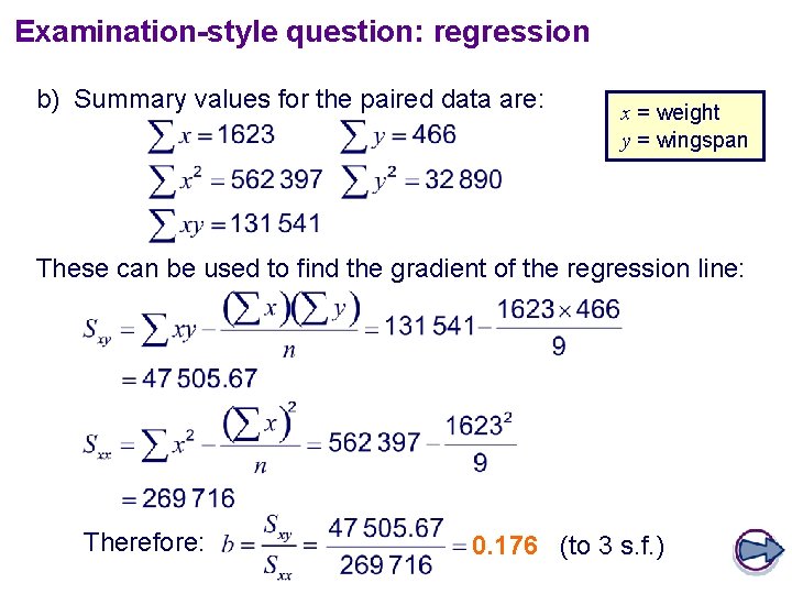
Examination-style question: regression b) Summary values for the paired data are: x = weight y = wingspan These can be used to find the gradient of the regression line: Therefore: 0. 176 (to 3 s. f. )

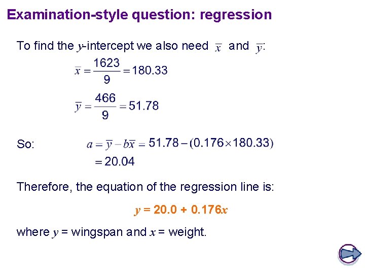
Examination-style question: regression To find the y-intercept we also need and : So: Therefore, the equation of the regression line is: y = 20. 0 + 0. 176 x where y = wingspan and x = weight.

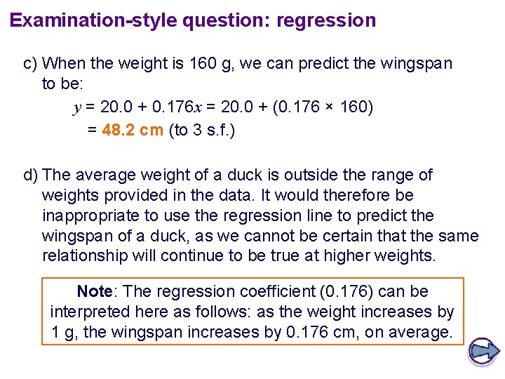
Examination-style question: regression c) When the weight is 160 g, we can predict the wingspan to be: y = 20. 0 + 0. 176 x = 20. 0 + (0. 176 × 160) = 48. 2 cm (to 3 s. f. ) d) The average weight of a duck is outside the range of weights provided in the data. It would therefore be inappropriate to use the regression line to predict the wingspan of a duck, as we cannot be certain that the same relationship will continue to be true at higher weights. Note: The regression coefficient (0. 176) can be interpreted here as follows: as the weight increases by 1 g, the wingspan increases by 0. 176 cm, on average.