Regression Control Charting Using the Random Coefficient Regression

Regression Control Charting Using the Random Coefficient Regression Method 22 March 2017 – JMP® Discovery Summit Europe 2017 Marriott Hotel, Prague Pius Dahinden, Manager Analytical Science at Tillotts Pharma AG, Switzerland Regression Control Chart Using the Random Coefficient Regression Method | 1 / 21

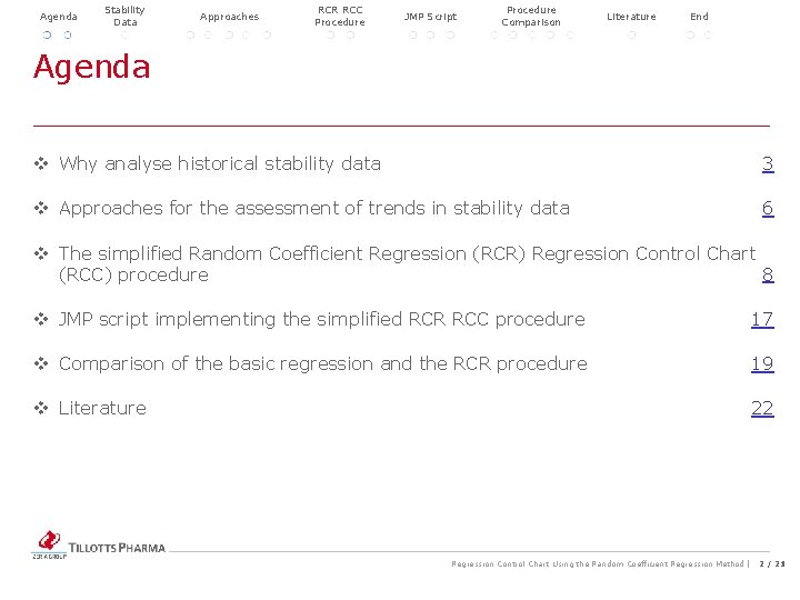
Agenda Stability Data Agenda Approaches RCR RCC Procedure JMP Script Procedure Comparison Literature End v Why analyse historical stability data 3 v Approaches for the assessment of trends in stability data 6 v The simplified Random Coefficient Regression (RCR) Regression Control Chart (RCC) procedure 8 v JMP script implementing the simplified RCR RCC procedure 17 v Comparison of the basic regression and the RCR procedure 19 v Literature 22 Regression Control Chart Using the Random Coefficient Regression Method | 2 / 21

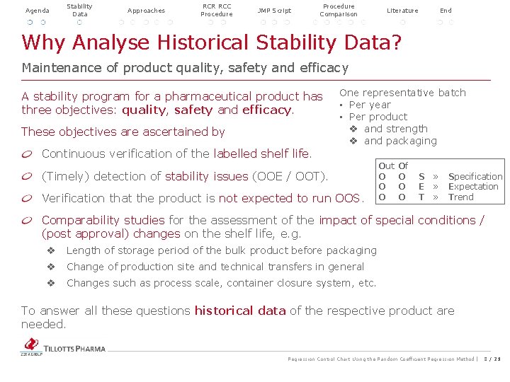
Agenda Stability Data Approaches RCR RCC Procedure JMP Script Procedure Comparison Literature Why Analyse Historical Stability Data? End Maintenance of product quality, safety and efficacy A stability program for a pharmaceutical product has three objectives: quality, safety and efficacy. These objectives are ascertained by One representative batch • Per year • Per product v and strength v and packaging Continuous verification of the labelled shelf life. (Timely) detection of stability issues (OOE / OOT). Verification that the product is not expected to run OOS. Out O Of O O O S » Specification E » Expectation T » Trend Comparability studies for the assessment of the impact of special conditions / (post approval) changes on the shelf life, e. g. v Length of storage period of the bulk product before packaging v Change of production site and technical transfers in general v Changes such as process scale, container closure system, etc. To answer all these questions historical data of the respective product are needed. Regression Control Chart Using the Random Coefficient Regression Method | 3 / 21

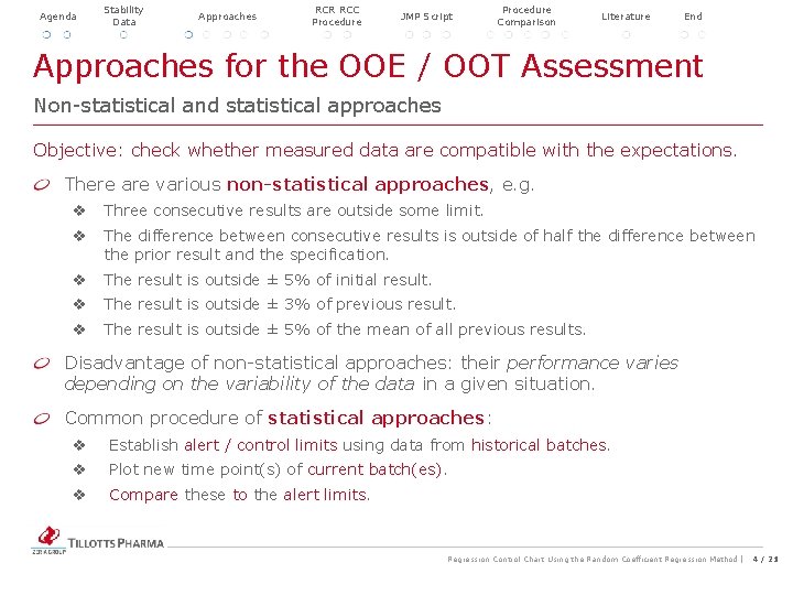
Agenda Stability Data Approaches RCR RCC Procedure Comparison JMP Script Literature End Approaches for the OOE / OOT Assessment Non-statistical and statistical approaches Objective: check whether measured data are compatible with the expectations. There are various non-statistical approaches, e. g. v Three consecutive results are outside some limit. v The difference between consecutive results is outside of half the difference between the prior result and the specification. v The result is outside ± 5% of initial result. v The result is outside ± 3% of previous result. v The result is outside ± 5% of the mean of all previous results. Disadvantage of non-statistical approaches: their performance varies depending on the variability of the data in a given situation. Common procedure of statistical approaches: v Establish alert / control limits using data from historical batches. v Plot new time point(s) of current batch(es). v Compare these to the alert limits. Regression Control Chart Using the Random Coefficient Regression Method | 4 / 21

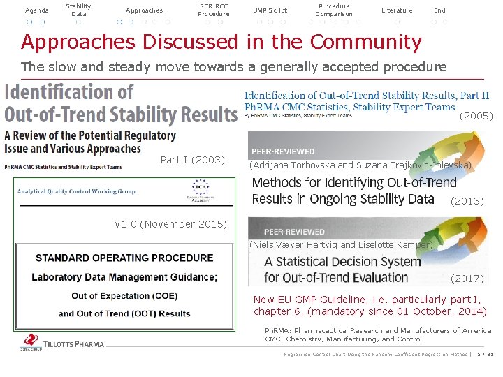
Agenda Stability Data Approaches RCR RCC Procedure JMP Script Procedure Comparison Literature Approaches Discussed in the Community End The slow and steady move towards a generally accepted procedure (2005) Part I (2003) (Adrijana Torbovska and Suzana Trajkovic-Jolevska) (2013) v 1. 0 (November 2015) (Niels Væver Hartvig and Liselotte Kamper) (2017) New EU GMP Guideline, i. e. particularly part I, chapter 6, (mandatory since 01 October, 2014) Ph. RMA: Pharmaceutical Research and Manufacturers of America CMC: Chemistry, Manufacturing, and Control Regression Control Chart Using the Random Coefficient Regression Method | 5 / 21

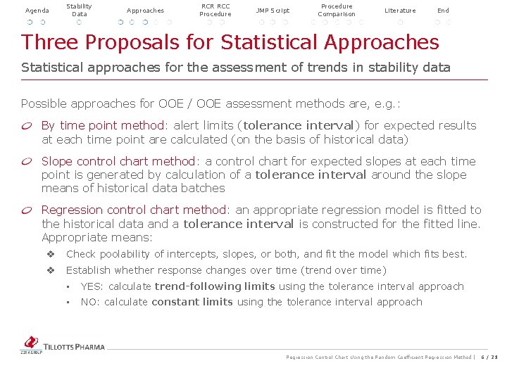
Agenda Stability Data Approaches RCR RCC Procedure JMP Script Procedure Comparison Literature End Three Proposals for Statistical Approaches Statistical approaches for the assessment of trends in stability data Possible approaches for OOE / OOE assessment methods are, e. g. : By time point method: alert limits (tolerance interval) for expected results at each time point are calculated (on the basis of historical data) Slope control chart method: a control chart for expected slopes at each time point is generated by calculation of a tolerance interval around the slope means of historical data batches Regression control chart method: an appropriate regression model is fitted to the historical data and a tolerance interval is constructed for the fitted line. Appropriate means: v Check poolability of intercepts, slopes, or both, and fit the model which fits best. v Establish whether response changes over time (trend over time) • YES: calculate trend-following limits using the tolerance interval approach • NO: calculate constant limits using the tolerance interval approach Regression Control Chart Using the Random Coefficient Regression Method | 6 / 21

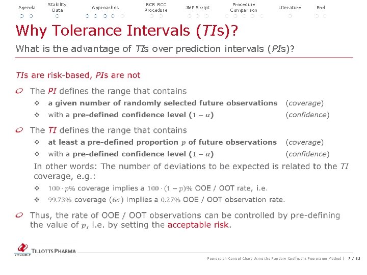
Agenda Stability Data Approaches RCR RCC Procedure JMP Script Procedure Comparison Why Tolerance Intervals (TIs)? Literature End What is the advantage of TIs over prediction intervals (PIs)? Regression Control Chart Using the Random Coefficient Regression Method | 7 / 21

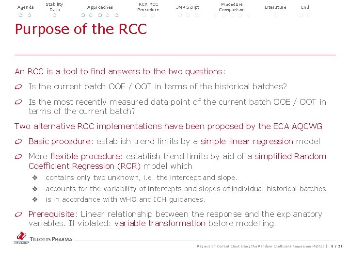
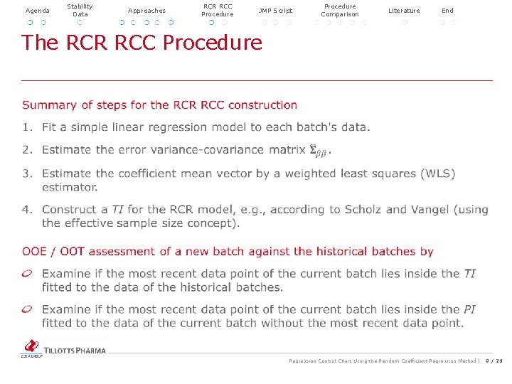
Agenda Stability Data Approaches RCR RCC Procedure Purpose of the RCC JMP Script Procedure Comparison Literature End An RCC is a tool to find answers to the two questions: Is the current batch OOE / OOT in terms of the historical batches? Is the most recently measured data point of the current batch OOE / OOT in terms of the current batch? Two alternative RCC implementations have been proposed by the ECA AQCWG Basic procedure: establish trend limits by a simple linear regression model More flexible procedure: establish trend limits by aid of a simplified Random Coefficient Regression (RCR) model which v contains only two unknown, i. e. the intercept and slope. v accounts for the variability of intercepts and slopes of individual historical batches. v is in accordance with WHO and ICH guidances. Prerequisite: Linear relationship between the response and the explanatory variables. If violated: variable transformation before modelling. Regression Control Chart Using the Random Coefficient Regression Method | 8 / 21

Agenda Stability Data Approaches RCR RCC Procedure JMP Script The RCR RCC Procedure Comparison Literature End Regression Control Chart Using the Random Coefficient Regression Method | 9 / 21

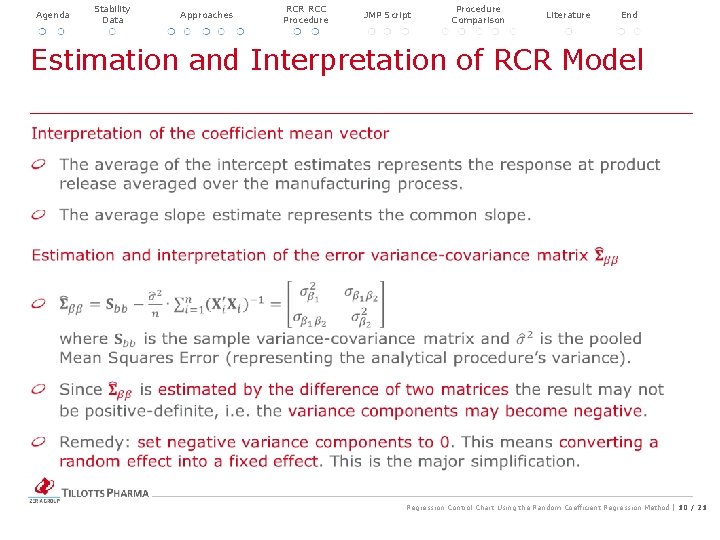
Agenda Stability Data Approaches RCR RCC Procedure JMP Script Procedure Comparison Literature End Estimation and Interpretation of RCR Model Regression Control Chart Using the Random Coefficient Regression Method | 10 / 21

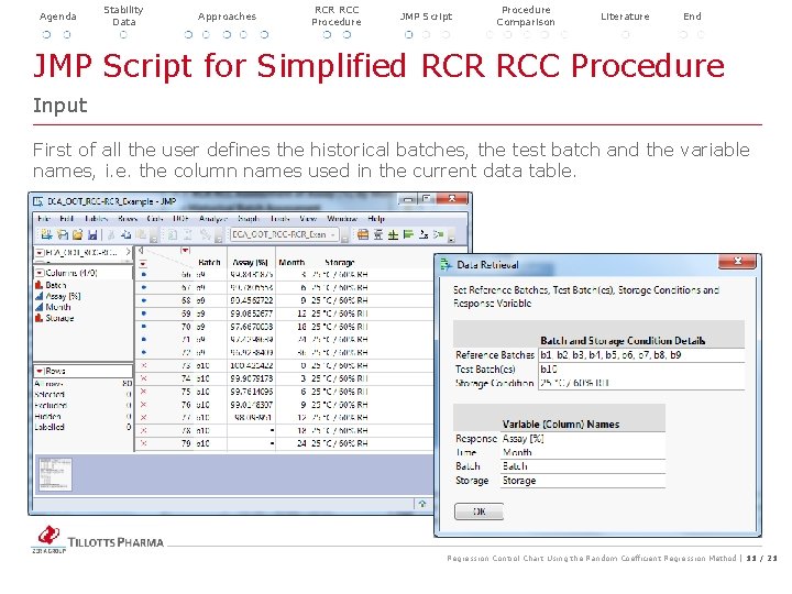
Agenda Stability Data Approaches RCR RCC Procedure JMP Script Procedure Comparison Literature End JMP Script for Simplified RCR RCC Procedure Input First of all the user defines the historical batches, the test batch and the variable names, i. e. the column names used in the current data table. Regression Control Chart Using the Random Coefficient Regression Method | 11 / 21

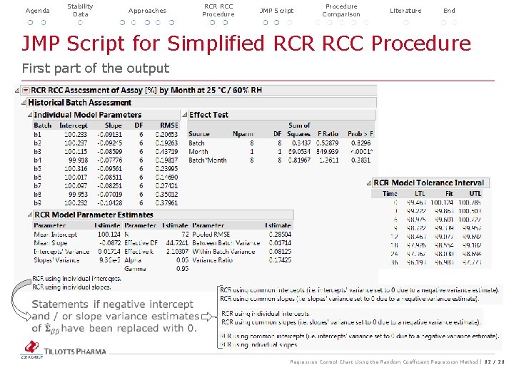
Agenda Stability Data Approaches RCR RCC Procedure JMP Script Procedure Comparison Literature End JMP Script for Simplified RCR RCC Procedure First part of the output Regression Control Chart Using the Random Coefficient Regression Method | 12 / 21

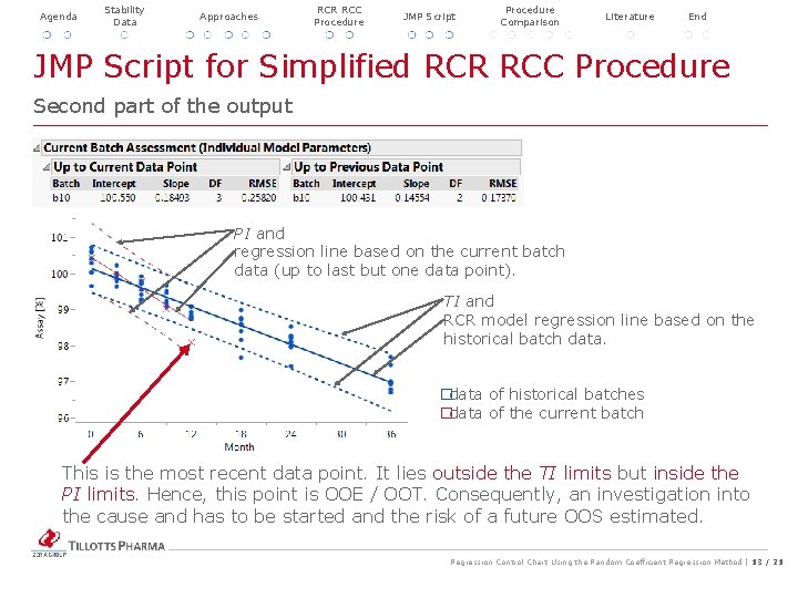
Agenda Stability Data Approaches RCR RCC Procedure JMP Script Procedure Comparison Literature End JMP Script for Simplified RCR RCC Procedure Second part of the output PI and regression line based on the current batch data (up to last but one data point). TI and RCR model regression line based on the historical batch data. � data of historical batches � data of the current batch This is the most recent data point. It lies outside the TI limits but inside the PI limits. Hence, this point is OOE / OOT. Consequently, an investigation into the cause and has to be started and the risk of a future OOS estimated. Regression Control Chart Using the Random Coefficient Regression Method | 13 / 21

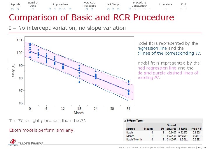
Agenda Stability Data Approaches RCR RCC Procedure JMP Script Procedure Comparison Literature Comparison of Basic and RCR Procedure End I – No intercept variation, no slope variation The RCR model fit is represented by the blue solid regression line and the blue dotted lines of the corresponding TI. The basic model fit is represented by the purple dashed regression line and the purple shade and purple dashed lines of the corresponding PI. The TI is slightly broader than the PI. � both models perform similarly. Regression Control Chart Using the Random Coefficient Regression Method | 14 / 21

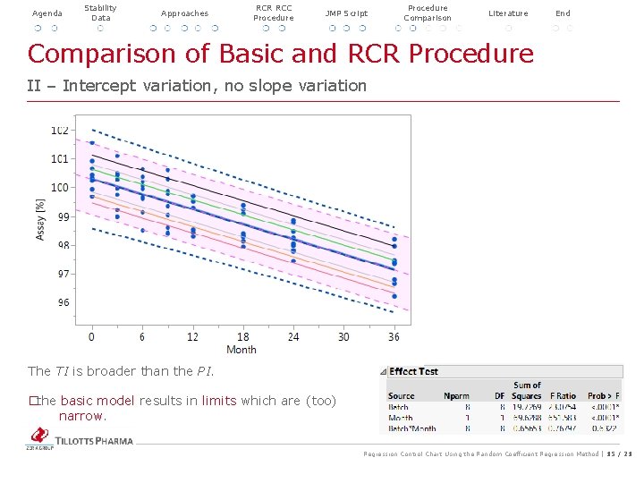
Agenda Stability Data Approaches RCR RCC Procedure JMP Script Procedure Comparison Literature Comparison of Basic and RCR Procedure End II – Intercept variation, no slope variation The TI is broader than the PI. � the basic model results in limits which are (too) narrow. Regression Control Chart Using the Random Coefficient Regression Method | 15 / 21

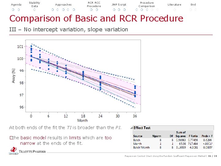
Agenda Stability Data Approaches RCR RCC Procedure JMP Script Procedure Comparison Literature Comparison of Basic and RCR Procedure End III – No intercept variation, slope variation At both ends of the fit the TI is broader than the PI. � the basic model results in limits which are too narrow at the ends of the fit. Regression Control Chart Using the Random Coefficient Regression Method | 16 / 21

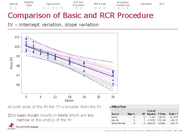
Agenda Stability Data Approaches RCR RCC Procedure JMP Script Procedure Comparison Literature Comparison of Basic and RCR Procedure End IV – intercept variation, slope variation At both ends of the fit the TI is broader than the PI. � the basic model results in limits which are too narrow at the end(s) of the fit Regression Control Chart Using the Random Coefficient Regression Method | 17 / 21

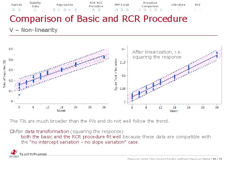
Agenda Stability Data Approaches RCR RCC Procedure JMP Script Procedure Comparison Literature Comparison of Basic and RCR Procedure End V – Non-linearity After linearization, i. e. squaring the response The TIs are much broader than the PIs and do not well follow the trend. � After data transformation (squaring the response) both the basic and the RCR procedure fit well because these data are compatible with the “no intercept variation – no slope variation” case. Regression Control Chart Using the Random Coefficient Regression Method | 18 / 21

Agenda Stability Data Literature Approaches RCR RCC Procedure JMP Script Procedure Comparison Literature End 1. Bederman, S. S. Estimation Methods in Random Coefficient Regression for Continuous and Binary Longitudinal Data. University of Toronto (1997). LINK 2. Carter, R. L, and Yang, M. C. K. Large sample inference in random coefficient regression models. Communications in Statistics – Theory and Methods (1986) 15(8): 2507 -2525. LINK 3. ICH Guidance Q 1 A(R 2), Stability Testing of New Drug Substances and Product, step 4 version, 6 February 2003. LINK 4. Mandel, B. J. Regression Control Chart. J Qual Technol (1969) 1(1): 1 -9. LINK 5. Scholz, F. , and Vangel, M. Tolerance bounds and Cpk confidence bounds under batch effects. Published in: Advanced in Stochastic Models for Reliability, Quality and Safety. Edited by Kahle, W. , von Collani, E. , Franz, J. , and Jensen, U. Birkhäuser, Boston, 1998, 361 -379. LINK 6. Shewhart, W. A. (1939). Statistical method from the viewpoint of quality control. (Deming, W. E. ). Washington, D. C. , The Graduate School, the Department of Agriculture. 7. Standard Operating Procedure – Laboratory Data Management Guidance – Out of Expecteation (OOE) and Out of Trend (OOT) Results. European Compliance Academy (ECA) Analytical Quality Control Working Group, Christopher Burgess, v 1. 0, 2015 (rev 8). 8. Torbovska, A. , Trajkovic-Jolevska, S. Methods for Identifying Out-of-Trend Results in Ongoing Stability Data. Pharm Tech Europe (2013) 37(6): 38 -42. LINK 9. WHO technical report series, No. 953, Annex 2 Stability testing of active pharmaceutical ingredients and finished pharmaceutical products, 2009. LINK Regression Control Chart Using the Random Coefficient Regression Method | 19 / 21

Agenda Stability Data Approaches Questions RCR RCC Procedure JMP Script Procedure Comparison Literature End Thank you for your attention! Regression Control Chart Using the Random Coefficient Regression Method | 20 / 21

Regression Control Chart Using the Random Coefficient Regression Method | 21 / 21

Part with Supplementary Information Regression Control Chart Using the Random Coefficient Regression Method | 22 / 21

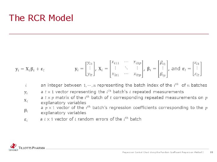
The RCR Model Regression Control Chart Using the Random Coefficient Regression Method | 23

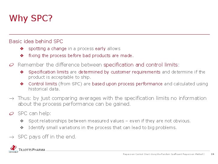
Why SPC? Basic idea behind SPC v spotting a change in a process early allows v fixing the process before bad products are made. Remember the difference between specification and control limits: v Specification limits are determined by customer requirements and determine if the product is acceptable to ship. v Control limits (from SPC) are based upon process performance and calculated using historical data. ® Thus: by just comparing averages with the specification limits no information about the process performance can be gained. SPC can help: v Spot relationships between measured values – even if they are not obvious. v Identify small variations in the process that can lead to big problems. ® SPC pays off in the end. Regression Control Chart Using the Random Coefficient Regression Method | 24

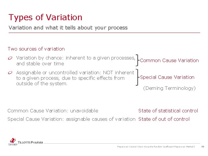
Types of Variation and what it tells about your process Two sources of variation Variation by chance: inherent to a given processes, Common Cause Variation and stable over time Assignable or uncontrolled variation: NOT inherent Special Cause Variation to a given process, due to specific effects from outside of the system. (Deming Terminology) Common Cause Variation: unavoidable State of statistical control Special Cause Variation: assignable causes of variation State of out of control Regression Control Chart Using the Random Coefficient Regression Method | 25

Basic Principles Reasons for usefulness of control charts Process Stability Stable process: common cause variation only. Typical fix (if too high): redesign the process. Unstable process: mean shift, spike or trend in data. Typical fix: eliminate cause and bring back into control. Control Charts designed by Shewhart intend to Distinguish between common and special causes of variation within a process. Minimize the risk of confusing common and special causes. Early detect process instability to be able to take corrective action before process runs out of control. Regression Control Chart Using the Random Coefficient Regression Method | 26

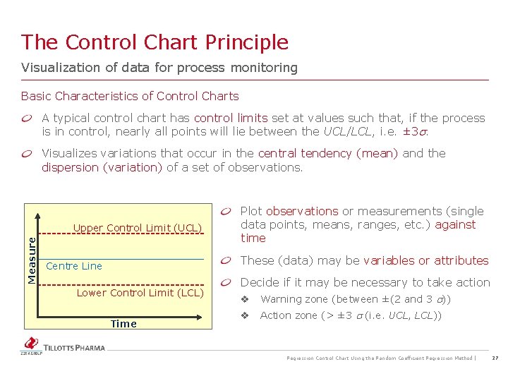
The Control Chart Principle Visualization of data for process monitoring Basic Characteristics of Control Charts A typical control chart has control limits set at values such that, if the process is in control, nearly all points will lie between the UCL/LCL, i. e. ± 3 s. Visualizes variations that occur in the central tendency (mean) and the dispersion (variation) of a set of observations. Measure Upper Control Limit (UCL) Plot observations or measurements (single data points, means, ranges, etc. ) against time These (data) may be variables or attributes Centre Line Lower Control Limit (LCL) Time Decide if it may be necessary to take action v Warning zone (between ±(2 and 3 s)) v Action zone (> ± 3 s (i. e. UCL, LCL)) Regression Control Chart Using the Random Coefficient Regression Method | 27

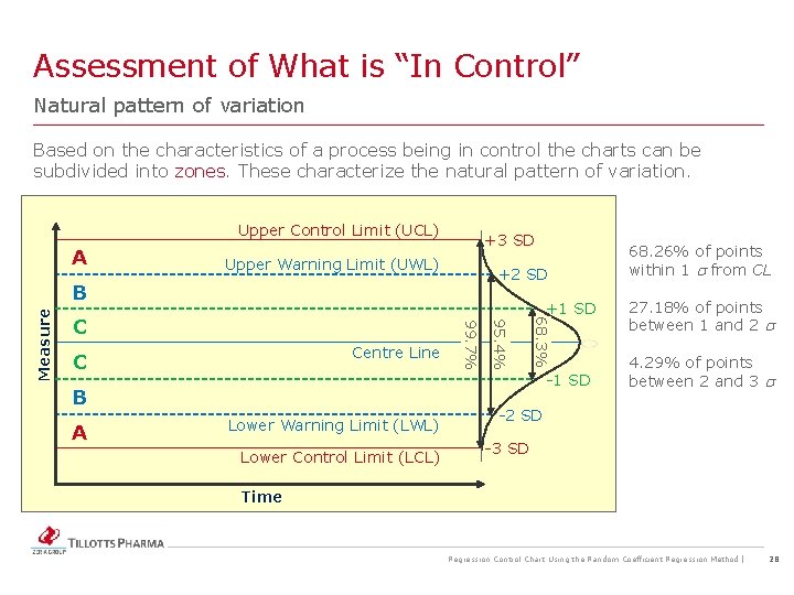
Assessment of What is “In Control” Natural pattern of variation Based on the characteristics of a process being in control the charts can be subdivided into zones. These characterize the natural pattern of variation. Upper Control Limit (UCL) A +3 SD Upper Warning Limit (UWL) +2 SD B Lower Warning Limit (LWL) Lower Control Limit (LCL) 27. 18% of points between 1 and 2 s Centre Line C 95. 4% C 68. 3% +1 SD 99. 7% Measure B A 68. 26% of points within 1 s from CL -1 SD 4. 29% of points between 2 and 3 s -2 SD -3 SD Time Regression Control Chart Using the Random Coefficient Regression Method | 28

Concepts Subgroups and Limits Subgroup Concept Data are collected over time in subgroups, where a subgroup is: v A number of consecutive samples (e. g. 3 to 5*) period (hour, day, shift, etc. ). In this case, the subgroup size is 3 to 5. v One single sample period. Thus, the subgroup size is 1. v Defect rate period. Here, the subgroup size is the number of service or units produced period. * Note: the subgroup size has no upper limit. Limits Specification Limits (SL) v Are used to evaluate process capability. v SLs tell us how well the product meets customer expectations. Control Limits (CL) v Are used to evaluate process stability. v CLs should warn of process instability. On the other hand you don’t want to have too many false alarms. Regression Control Chart Using the Random Coefficient Regression Method | 29

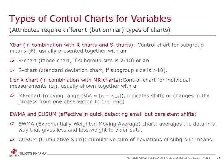
Types of Control Charts for Variables (Attributes require different (but similar) types of charts) Regression Control Chart Using the Random Coefficient Regression Method | 30

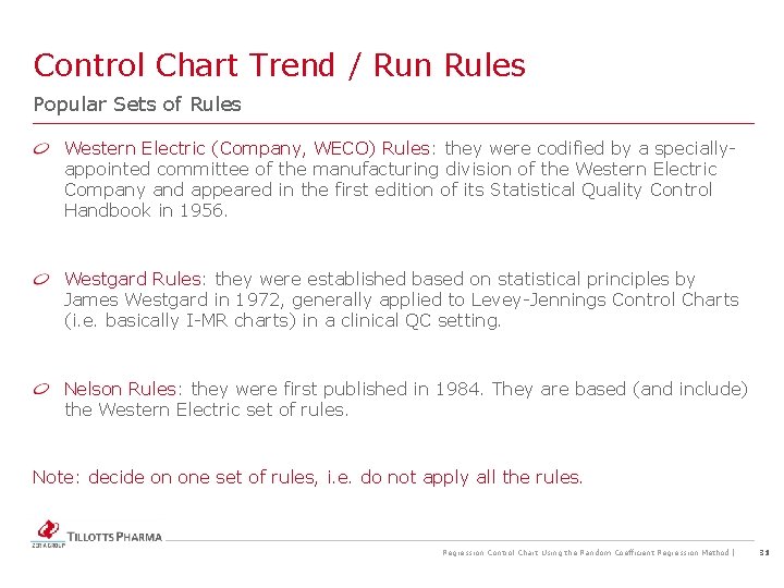
Control Chart Trend / Run Rules Popular Sets of Rules Western Electric (Company, WECO) Rules: they were codified by a speciallyappointed committee of the manufacturing division of the Western Electric Company and appeared in the first edition of its Statistical Quality Control Handbook in 1956. Westgard Rules: they were established based on statistical principles by James Westgard in 1972, generally applied to Levey-Jennings Control Charts (i. e. basically I-MR charts) in a clinical QC setting. Nelson Rules: they were first published in 1984. They are based (and include) the Western Electric set of rules. Note: decide on one set of rules, i. e. do not apply all the rules. Regression Control Chart Using the Random Coefficient Regression Method | 31

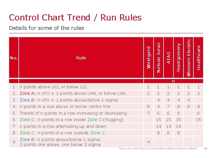
Control Chart Trend / Run Rules Western Electric Healthcare 1 1 1 2 Zone A; n of n + 1 points above UWL or below LWL 2 2 2 3 Zone B: n of n + 1 points above/below 1 sigma 4 4 4 n points in a row above or below centre line 8 9 7 8 8 5 Trends of n points in a row increasing or decreasing 7 6 6 6 Zone C: n points in a row inside Zone C (hugging) 15 15 7 n points in a row alternating up and down 14 14 14 8 Zone C: n points in a row outside Zone C 8 8 8 9 Zone B: n points above/below 1 sigma; 2 points one above, one below 2 sigma AIAG n points above UCL or below LCL Rule Nelson Juran 1 No. Westgard Montgomery Details for some of the rules n 8 4 Regression Control Chart Using the Random Coefficient Regression Method | 32

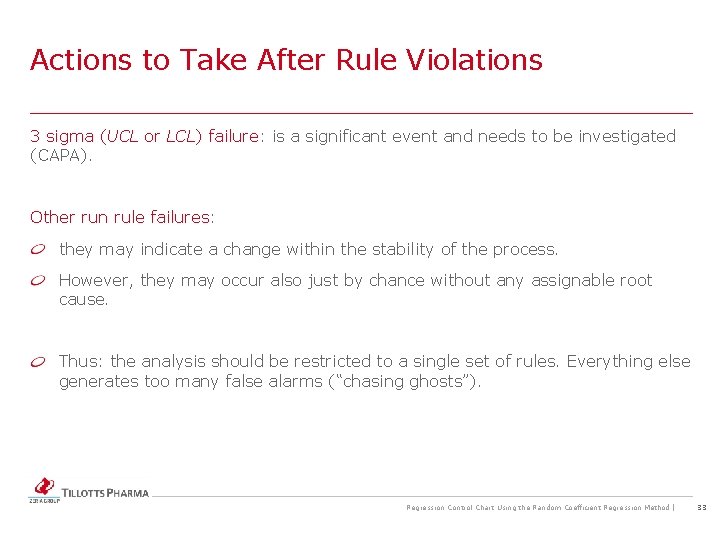
Actions to Take After Rule Violations 3 sigma (UCL or LCL) failure: is a significant event and needs to be investigated (CAPA). Other run rule failures: they may indicate a change within the stability of the process. However, they may occur also just by chance without any assignable root cause. Thus: the analysis should be restricted to a single set of rules. Everything else generates too many false alarms (“chasing ghosts”). Regression Control Chart Using the Random Coefficient Regression Method | 33

Regression Control Chart Using the Random Coefficient Regression Method | 34 / 21