Regression Analysis With a Categorical Dependent Variable Basic

Regression Analysis With a Categorical Dependent Variable Basic Logistic Regression (“Binomial Logit”) Analysis • Source: http: //icommons. harvard. edu/~gse-s 052/ Slide 1

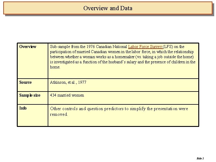
Overview and Data Overview Sub-sample from the 1976 Canadian National Labor Force Survey (LFS) on the participation of married Canadian women in the labor force, in which the relationship between whether a woman works as a homemaker (vs. taking a job outside the home) is investigated as a function of the husband’s salary and the presence of children in the home. Source Atkinson, et al. , 1977 Sample size 434 married women Info Other controls and question predictors to simplify the presentation were removed. Slide 2

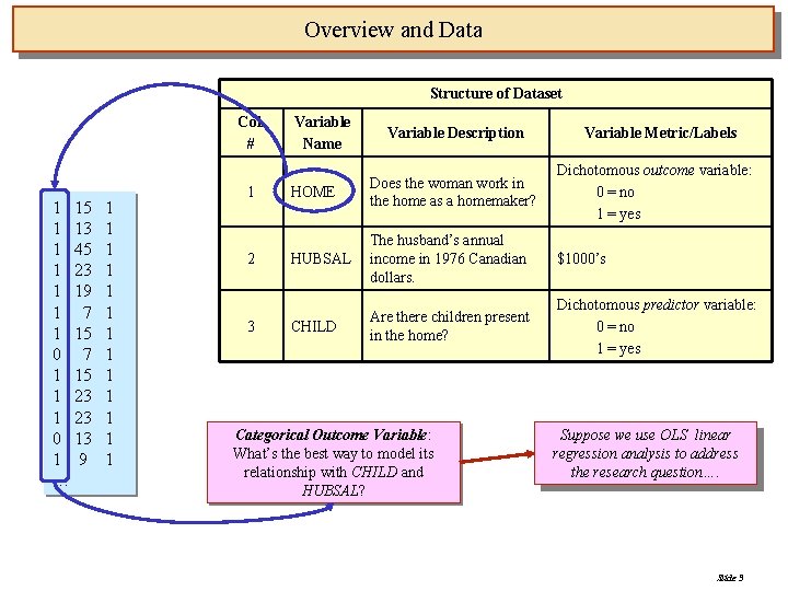
Overview and Data Structure of Dataset Col. # 1 15 1 13 1 45 1 23 1 19 1 7 1 15 0 7 1 15 1 23 0 13 1 9 … 1 1 1 1 2 3 Variable Name Variable Description Variable Metric/Labels HOME Does the woman work in the home as a homemaker? Dichotomous outcome variable: 0 = no 1 = yes HUBSAL The husband’s annual income in 1976 Canadian dollars. $1000’s CHILD Are there children present in the home? Dichotomous predictor variable: 0 = no 1 = yes Categorical Outcome Variable: What’s the best way to model its relationship with CHILD and HUBSAL? Suppose we use OLS linear regression analysis to address the research question…. Slide 3

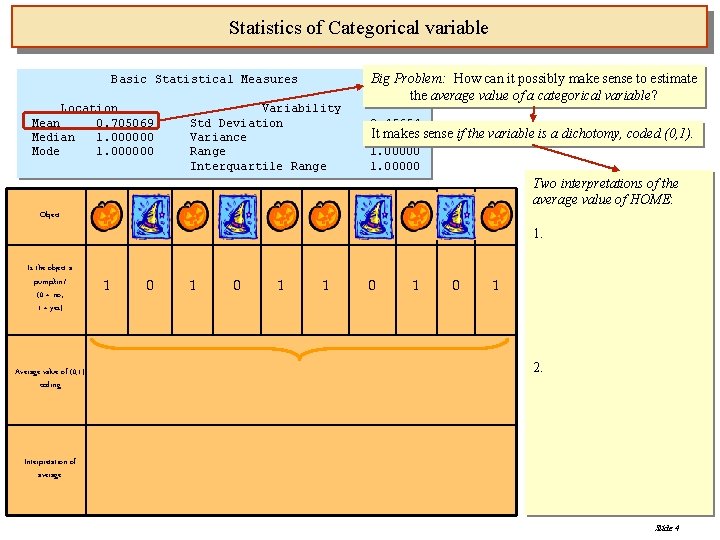
Statistics of Categorical variable Basic Statistical Measures Location Mean 0. 705069 Median 1. 000000 Mode 1. 000000 Variability Std Deviation Variance Range Interquartile Range Big Problem: How can it possibly make sense to estimate the average value of a categorical variable? 0. 45654 It makes sense if the variable is a dichotomy, coded (0, 1). 0. 20843 1. 00000 Two interpretations of the average value of HOME: Object 1. Is the object a pumpkin? (0 = no; 1 = yes) Average value of (0, 1) coding 1 0 1 0 1 2. Interpretation of average Slide 4

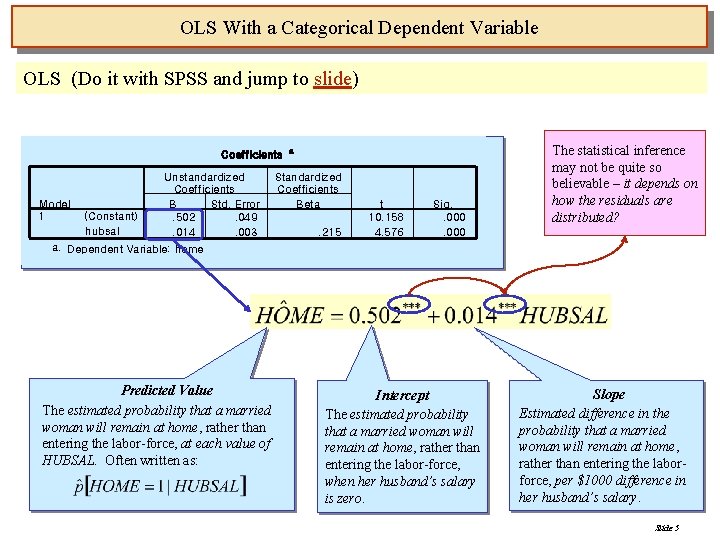
OLS With a Categorical Dependent Variable OLS (Do it with SPSS and jump to slide) Coefficients Model 1 (Constant) hubsal Unstandardized Coefficients B Std. Error. 502. 049. 014. 003 a Standardized Coefficients Beta. 215 t 10. 158 4. 576 Sig. . 000 The statistical inference may not be quite so believable – it depends on how the residuals are distributed? a. Dependent Variable: home Predicted Value The estimated probability that a married woman will remain at home, rather than entering the labor-force, at each value of HUBSAL. Often written as: Intercept The estimated probability that a married woman will remain at home, rather than entering the labor-force, when her husband’s salary is zero. Slope Estimated difference in the probability that a married woman will remain at home, rather than entering the laborforce, per $1000 difference in her husband’s salary. Slide 5

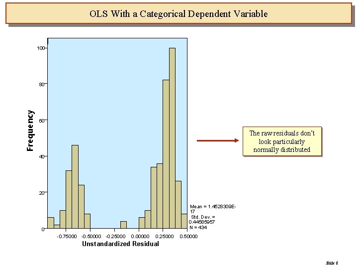
OLS With a Categorical Dependent Variable 100 Frequency 80 60 The raw residuals don’t look particularly normally distributed 40 20 Mean = 1. 4528309 E 17 Std. Dev. = 0. 44585957 N = 434 0 -0. 75000 -0. 50000 -0. 25000 0. 00000 0. 25000 0. 50000 Unstandardized Residual Slide 6

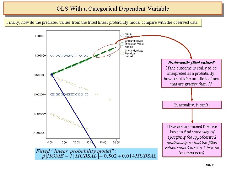
OLS With a Categorical Dependent Variable Finally, how do the predicted values from the fitted linear probability model compare with the observed data: Problematic fitted values? If the outcome is really to be interpreted as a probability, how can it take on fitted values that are greater than 1? In actuality, it can’t! If we are to proceed then we have to find some way of specifying the hypothesized relationship so that the fitted values cannot exceed 1 (nor be less than zero). Slide 7

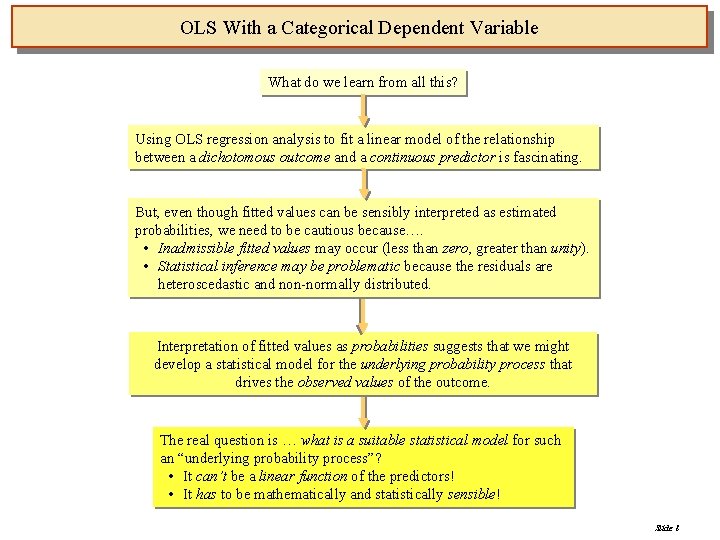
OLS With a Categorical Dependent Variable What do we learn from all this? Using OLS regression analysis to fit a linear model of the relationship between a dichotomous outcome and a continuous predictor is fascinating. But, even though fitted values can be sensibly interpreted as estimated probabilities, we need to be cautious because…. • Inadmissible fitted values may occur (less than zero, greater than unity). • Statistical inference may be problematic because the residuals are heteroscedastic and non-normally distributed. Interpretation of fitted values as probabilities suggests that we might develop a statistical model for the underlying probability process that drives the observed values of the outcome. The real question is … what is a suitable statistical model for such an “underlying probability process”? • It can’t be a linear function of the predictors! • It has to be mathematically and statistically sensible! Slide 8

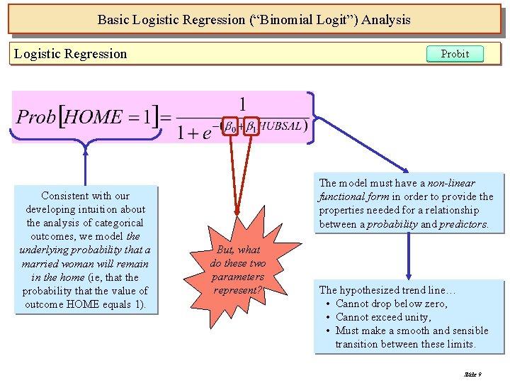
Basic Logistic Regression (“Binomial Logit”) Analysis Logistic Regression Consistent with our developing intuition about the analysis of categorical outcomes, we model the underlying probability that a married woman will remain in the home (ie, that the probability that the value of outcome HOME equals 1). Probit The model must have a non-linear functional form in order to provide the properties needed for a relationship between a probability and predictors. But, what do these two parameters represent? The hypothesized trend line… • Cannot drop below zero, • Cannot exceed unity, • Must make a smooth and sensible transition between these limits. Slide 9

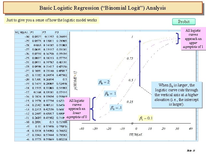
Basic Logistic Regression (“Binomial Logit”) Analysis Just to give you a sense of how the logistic model works Probit All logistic curves approach an upper asymptote of 1 All logistic curves approach an lower asymptote of 0 When 0 is larger, the logistic curve cuts through the vertical axis at a higher elevation (i. e. , the intercept is larger). Slide 10

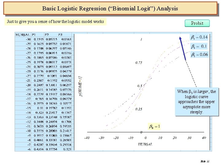
Basic Logistic Regression (“Binomial Logit”) Analysis Just to give you a sense of how the logistic model works Probit When 1 is larger, the logistic curve approaches the upper asymptote more steeply. Slide 11

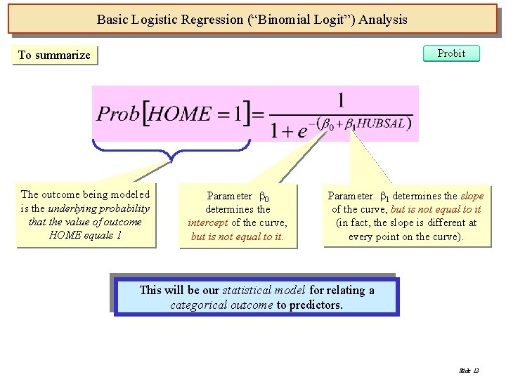
Basic Logistic Regression (“Binomial Logit”) Analysis Probit To summarize The outcome being modeled is the underlying probability that the value of outcome HOME equals 1 Parameter 0 determines the intercept of the curve, but is not equal to it. Parameter 1 determines the slope of the curve, but is not equal to it (in fact, the slope is different at every point on the curve). This will be our statistical model for relating a categorical outcome to predictors. Slide 12

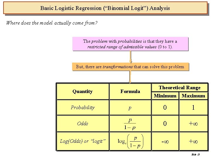
Basic Logistic Regression (“Binomial Logit”) Analysis Where does the model actually come from? The problem with probabilities is that they have a restricted range of admissible values (0 to 1). But, there are transformations that can solve this problem Quantity Formula Probability p Theoretical Range Minimum Maximum 0 1 Odds 0 + Log(Odds) or “logit” - + Slide 13

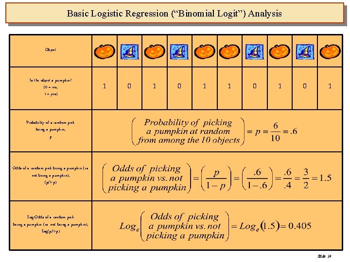
Basic Logistic Regression (“Binomial Logit”) Analysis Object Is the object a pumpkin? (0 = no; 1 = yes) 1 0 1 0 1 Probability of a random pick being a pumpkin, p Odds of a random pick being a pumpkin (vs. not being a pumpkin), (p/1 -p) Log-Odds of a random pick being a pumpkin (vs. not being a pumpkin), Log(p/1 -p) Slide 14

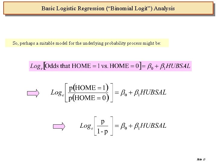
Basic Logistic Regression (“Binomial Logit”) Analysis So, perhaps a suitable model for the underlying probability process might be: Slide 15

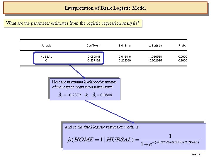
Interpretation of Basic Logistic Model What are the parameter estimates from the logistic regression analysis? Variable Coefficient Std. Error z-Statistic Prob. HUBSAL C 0. 080841 -0. 237192 0. 018416 0. 262690 4. 389588 -0. 902935 0. 0000 0. 3666 Here are maximum likelihood estimates of the logistic regression parameters: And so the fitted logistic regression model is: Slide 16

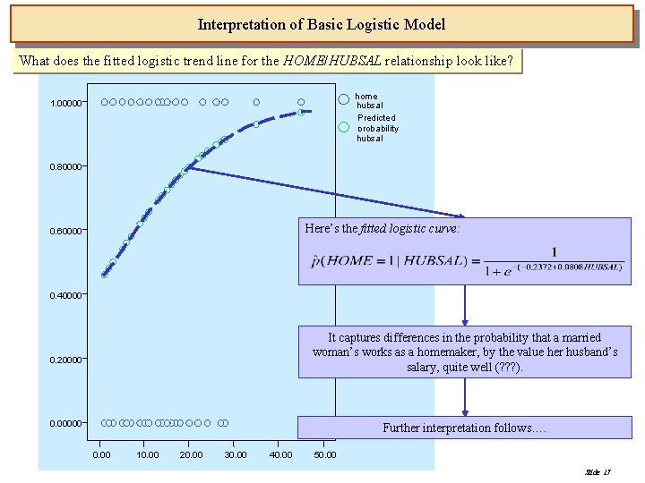
Interpretation of Basic Logistic Model What does the fitted logistic trend line for the HOME/HUBSAL relationship look like? home hubsal Predicted probability hubsal 1. 00000 0. 80000 Here’s the fitted logistic curve: 0. 60000 0. 40000 It captures differences in the probability that a married woman’s works as a homemaker, by the value her husband’s salary, quite well (? ? ? ). 0. 20000 0. 00000 Further interpretation follows…. 0. 00 10. 00 20. 00 30. 00 40. 00 50. 00 Slide 17

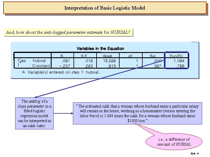
Interpretation of Basic Logistic Model And, how about the anti-logged parameter estimate for HUBSAL? Variables in the Equation B S. E. Wald Step hubsal. 081. 018 19. 268 a 1 Constant -. 237. 263. 815 a. Variable(s) entered on step 1: hubsal. The antilog of a slope parameter in a fitted logistic regression model can be interpreted as an odds-ratio: df 1 1 Sig. . 000. 367 Exp(B) 1. 084. 789 “The estimated odds that a woman whose husband earns a particular salary will remain in the home, working as a homemaker (versus entering the labor-force) is 1. 084 times the odds for a woman whose husband earns $1000 less. ” i. e. , a difference of one unit of HUBSAL Slide 18

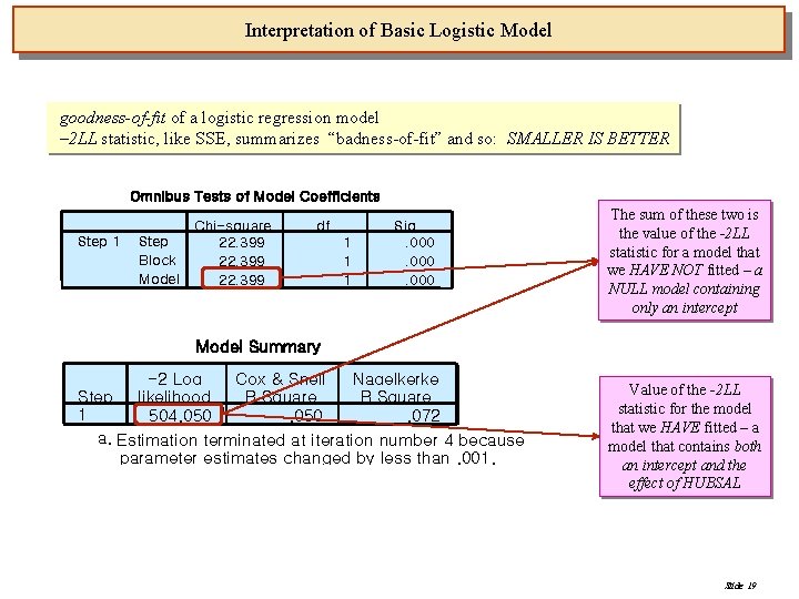
Interpretation of Basic Logistic Model goodness-of-fit of a logistic regression model – 2 LL statistic, like SSE, summarizes “badness-of-fit” and so: SMALLER IS BETTER Omnibus Tests of Model Coefficients Step 1 Step Block Model Chi-square 22. 399 df 1 1 1 Sig. . 000 The sum of these two is the value of the -2 LL statistic for a model that we HAVE NOT fitted – a NULL model containing only an intercept Model Summary -2 Log Cox & Snell Nagelkerke Step likelihood R Square a 1 504. 050. 072 a. Estimation terminated at iteration number 4 because parameter estimates changed by less than. 001. Value of the -2 LL statistic for the model that we HAVE fitted – a model that contains both an intercept and the effect of HUBSAL Slide 19

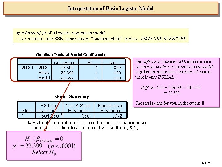
Interpretation of Basic Logistic Model goodness-of-fit of a logistic regression model – 2 LL statistic, like SSE, summarizes “badness-of-fit” and so: SMALLER IS BETTER Omnibus Tests of Model Coefficients Step 1 Step Block Model Chi-square 22. 399 df Model Summary 1 1 1 Sig. . 000 The difference between – 2 LL statistics tests whether all predictors currently in the model together are important (currently, of course, there is only HUBSAL) : Diff. In – 2 LL = 526. 449 – 504. 050 = 22. 399 The test is done for you, in the output!!! -2 Log Cox & Snell Nagelkerke Step likelihood R Square a 1 504. 050. 072 a. Estimation terminated at iteration number 4 because parameter estimates changed by less than. 001. Slide 20

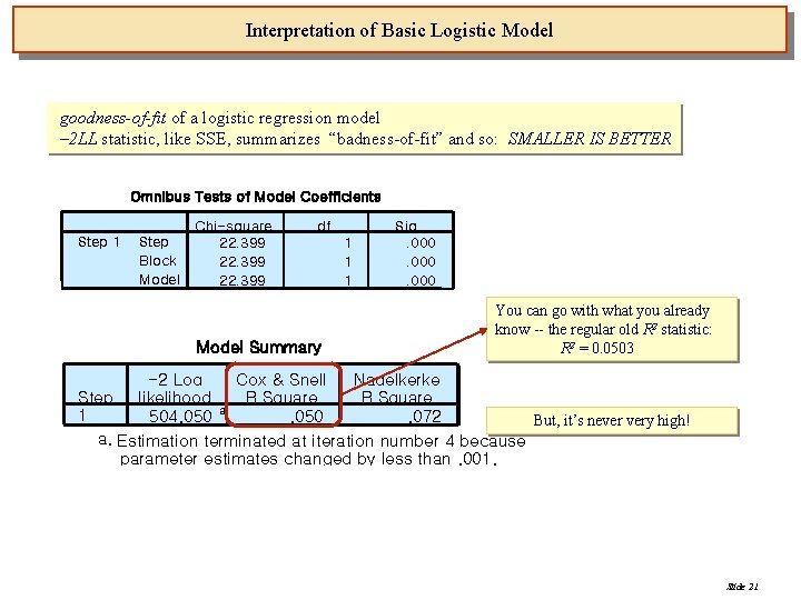
Interpretation of Basic Logistic Model goodness-of-fit of a logistic regression model – 2 LL statistic, like SSE, summarizes “badness-of-fit” and so: SMALLER IS BETTER Omnibus Tests of Model Coefficients Step 1 Step Block Model Chi-square 22. 399 df Model Summary 1 1 1 Sig. . 000 You can go with what you already know -- the regular old R 2 statistic: R 2 = 0. 0503 -2 Log Cox & Snell Nagelkerke Step likelihood R Square a 1 504. 050. 072 But, it’s never very high! a. Estimation terminated at iteration number 4 because parameter estimates changed by less than. 001. Slide 21

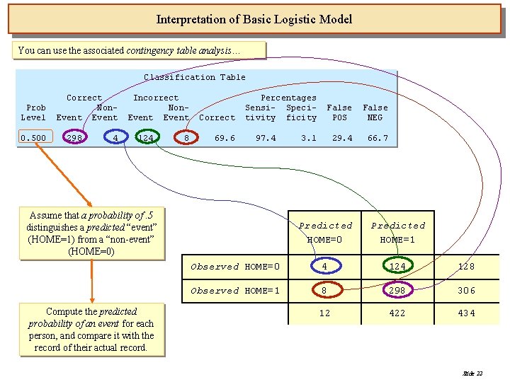
Interpretation of Basic Logistic Model You can use the associated contingency table analysis… Classification Table Prob Level 0. 500 Correct Non. Event 298 4 Incorrect Non. Event 124 8 Correct 69. 6 Percentages Sensi- Specitivity ficity 97. 4 Assume that a probability of. 5 distinguishes a predicted “event” (HOME=1) from a “non-event” (HOME=0) Compute the predicted probability of an event for each person, and compare it with the record of their actual record. False POS False NEG 29. 4 66. 7 3. 1 Predicted HOME=0 Predicted HOME=1 Observed HOME=0 4 128 Observed HOME=1 8 298 306 12 422 434 Slide 22

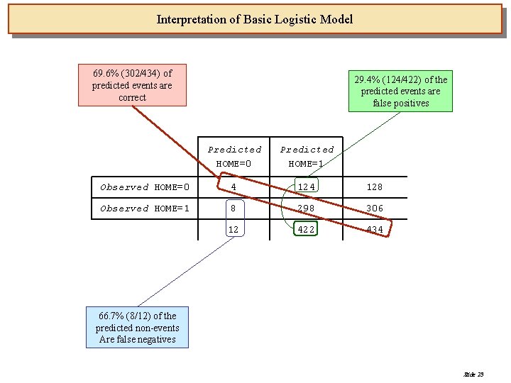
Interpretation of Basic Logistic Model 69. 6% (302/434) of predicted events are correct 29. 4% (124/422) of the predicted events are false positives Predicted HOME=0 Predicted HOME=1 Observed HOME=0 4 128 Observed HOME=1 8 298 306 12 422 434 66. 7% (8/12) of the predicted non-events Are false negatives Slide 23

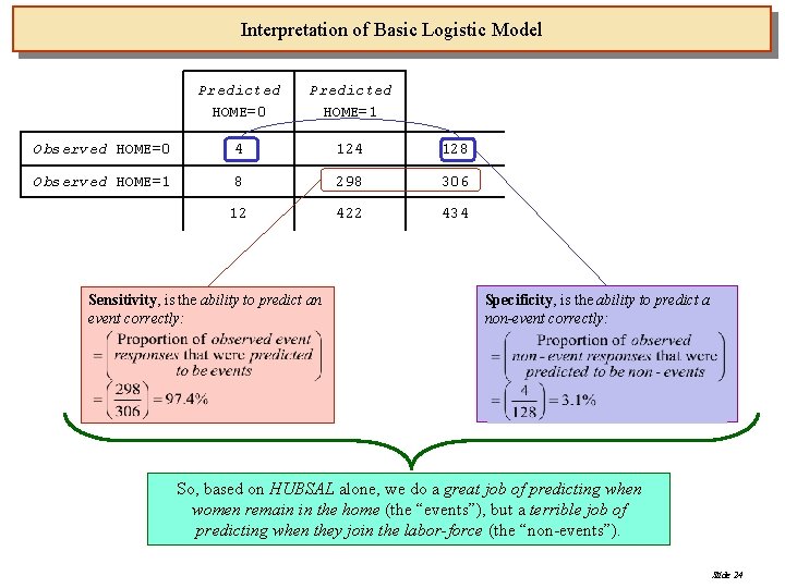
Interpretation of Basic Logistic Model Predicted HOME=0 Predicted HOME=1 Observed HOME=0 4 128 Observed HOME=1 8 298 306 12 422 434 Sensitivity, is the ability to predict an event correctly: Specificity, is the ability to predict a non-event correctly: So, based on HUBSAL alone, we do a great job of predicting when women remain in the home (the “events”), but a terrible job of predicting when they join the labor-force (the “non-events”). Slide 24

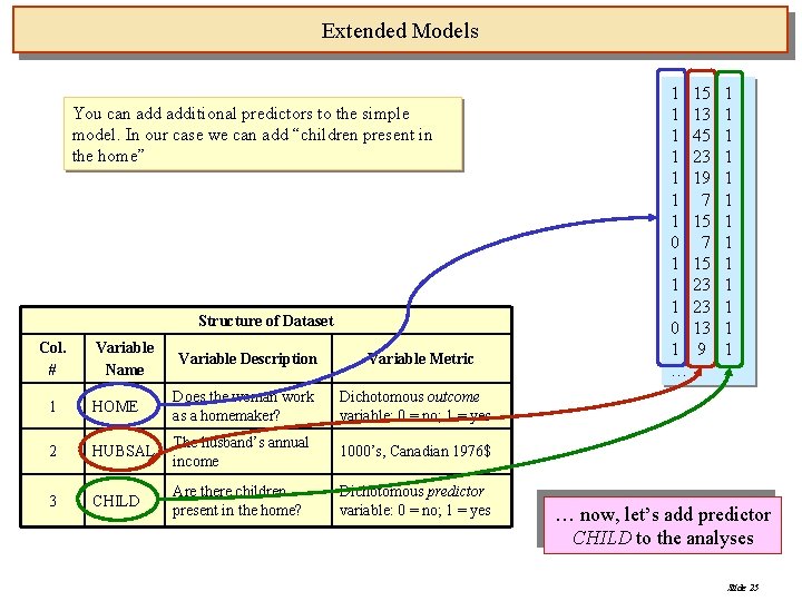
Extended Models You can additional predictors to the simple model. In our case we can add “children present in the home” Structure of Dataset Col. # Variable Name Variable Description Variable Metric 1 HOME Does the woman work as a homemaker? Dichotomous outcome variable: 0 = no; 1 = yes 2 HUBSAL The husband’s annual income 1000’s, Canadian 1976$ 3 CHILD Are there children present in the home? Dichotomous predictor variable: 0 = no; 1 = yes 1 15 1 13 1 45 1 23 1 19 1 7 1 15 0 7 1 15 1 23 0 13 1 9 … 1 1 1 1 … now, let’s add predictor CHILD to the analyses Slide 25

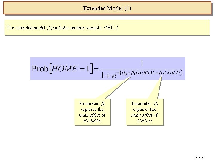
Extended Model (1) The extended model (1) includes another variable: CHILD. Parameter 1 captures the main effect of HUBSAL Parameter 2 captures the main effect of CHILD Slide 26

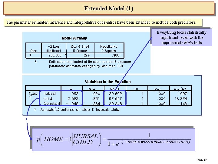
Extended Model (1) The parameter estimates, inference and interpretative odds-ratios have been extended to include both predictors… Everything looks statistically significant, even with the approximate Wald tests Model Summary Step 1 a. -2 Log likelihood 388. 086 a Cox & Snell R Square. 273 Nagelkerke R Square. 388 Estimation terminated at iteration number 5 because parameter estimates changed by less than. 001. Variables in the Equation B S. E. Wald Step hubsal. 092. 020 20. 602 a 1 child 2. 582. 261 97. 647 Constant -1. 948. 354 30. 345 a. Variable(s) entered on step 1: hubsal, child. df 1 1 1 Sig. . 000 Exp(B) 1. 097 13. 224. 143 Slide 27

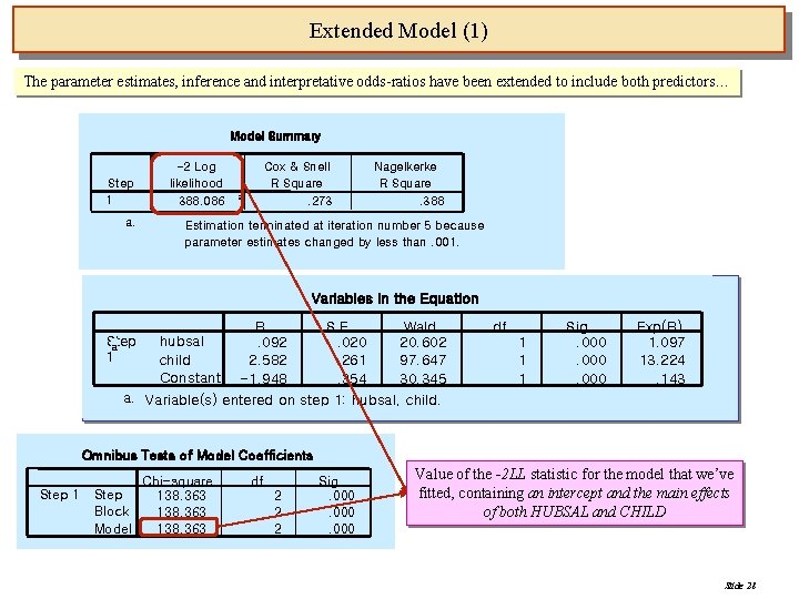
Extended Model (1) The parameter estimates, inference and interpretative odds-ratios have been extended to include both predictors… Model Summary Step 1 a. -2 Log likelihood 388. 086 Cox & Snell R Square. 273 a Nagelkerke R Square. 388 Estimation terminated at iteration number 5 because parameter estimates changed by less than. 001. Variables in the Equation B S. E. Wald Step hubsal. 092. 020 20. 602 a 1 child 2. 582. 261 97. 647 Constant -1. 948. 354 30. 345 a. Variable(s) entered on step 1: hubsal, child. df 1 1 1 Sig. . 000 Exp(B) 1. 097 13. 224. 143 Omnibus Tests of Model Coefficients Step 1 Chi-square Step 138. 363 Block 138. 363 Model 138. 363 df 2 2 2 Sig. . 000 Value of the -2 LL statistic for the model that we’ve fitted, containing an intercept and the main effects of both HUBSAL and CHILD Slide 28

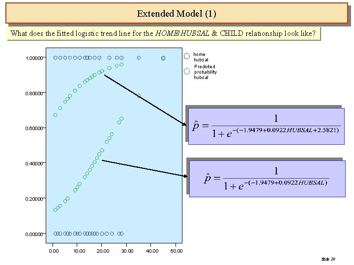
Extended Model (1) What does the fitted logistic trend line for the HOME/HUBSAL & CHILD relationship look like? home hubsal Predicted probability hubsal 1. 00000 0. 80000 0. 60000 0. 40000 0. 20000 0. 00 10. 00 20. 00 30. 00 40. 00 50. 00 Slide 29

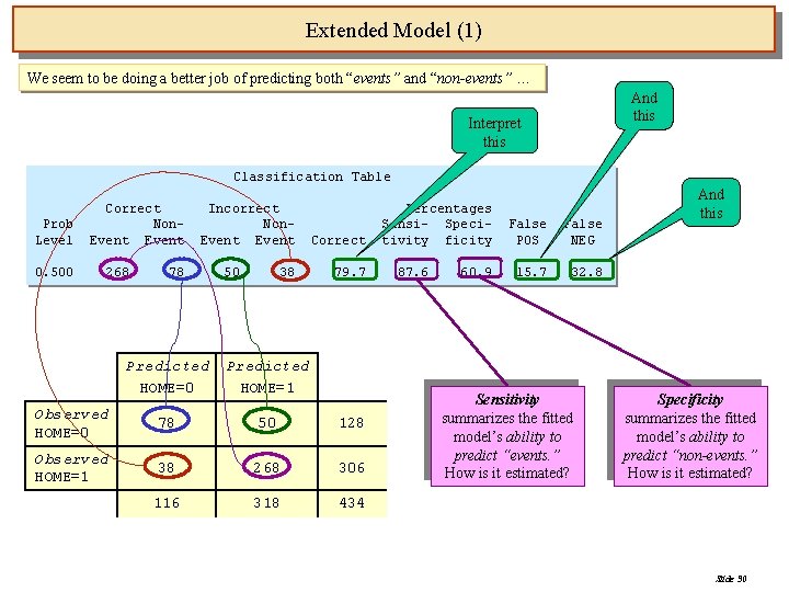
Extended Model (1) We seem to be doing a better job of predicting both “events” and “non-events” … And this Interpret this Classification Table Prob Level 0. 500 Correct Non. Event 268 Incorrect Non. Event 78 50 38 Correct 79. 7 Predicted HOME=0 Predicted HOME=1 Observed HOME=0 78 50 128 Observed HOME=1 38 268 306 116 318 434 Percentages Sensi- Specitivity ficity 87. 6 60. 9 False POS False NEG 15. 7 32. 8 Sensitivity summarizes the fitted model’s ability to predict “events. ” How is it estimated? And this Specificity summarizes the fitted model’s ability to predict “non-events. ” How is it estimated? Slide 30

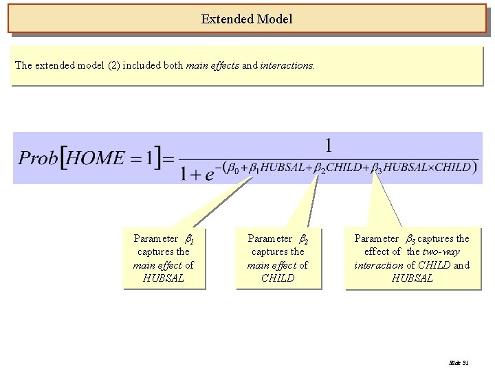
Extended Model The extended model (2) included both main effects and interactions. Parameter 1 captures the main effect of HUBSAL Parameter 2 captures the main effect of CHILD Parameter 3 captures the effect of the two-way interaction of CHILD and HUBSAL Slide 31

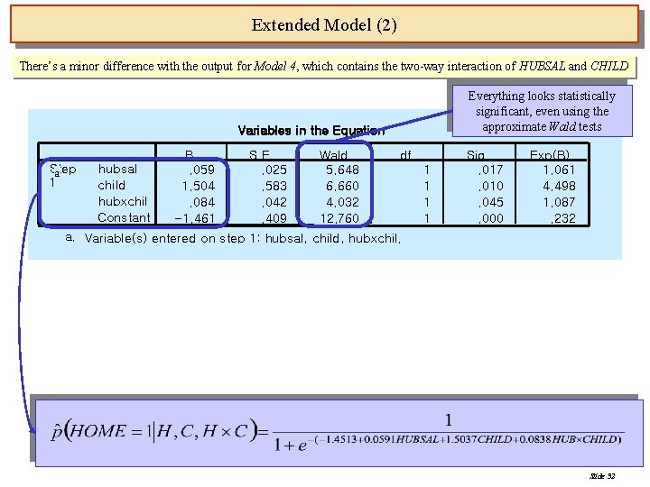
Extended Model (2) There’s a minor difference with the output for Model 4, which contains the two-way interaction of HUBSAL and CHILD Everything looks statistically significant, even using the approximate Wald tests Variables in the Equation Step a 1 hubsal child hubxchil Constant B. 059 1. 504. 084 -1. 461 S. E. . 025. 583. 042. 409 Wald 5. 648 6. 660 4. 032 12. 760 df 1 1 Sig. . 017. 010. 045. 000 Exp(B) 1. 061 4. 498 1. 087. 232 a. Variable(s) entered on step 1: hubsal, child, hubxchil. Slide 32

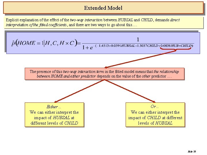
Extended Model Explicit explanation of the effect of the two-way interaction between HUBSAL and CHILD, demands direct interpretation of the fitted coefficients, and there are two ways to go about this…. The presence of this two-way interaction term in the fitted model means that the relationship between HOME and either predictor depends on the value of the other predictor …. Either… We can either interpret the impact of HUBSAL at different levels of CHILD Or… We can either interpret the impact of CHILD at different levels of HUBSAL Slide 33

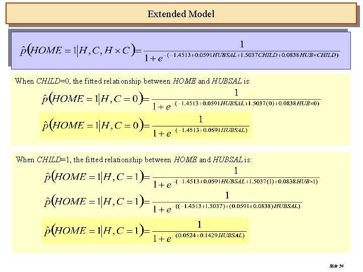
Extended Model When CHILD=0, the fitted relationship between HOME and HUBSAL is: When CHILD=1, the fitted relationship between HOME and HUBSAL is: Slide 34

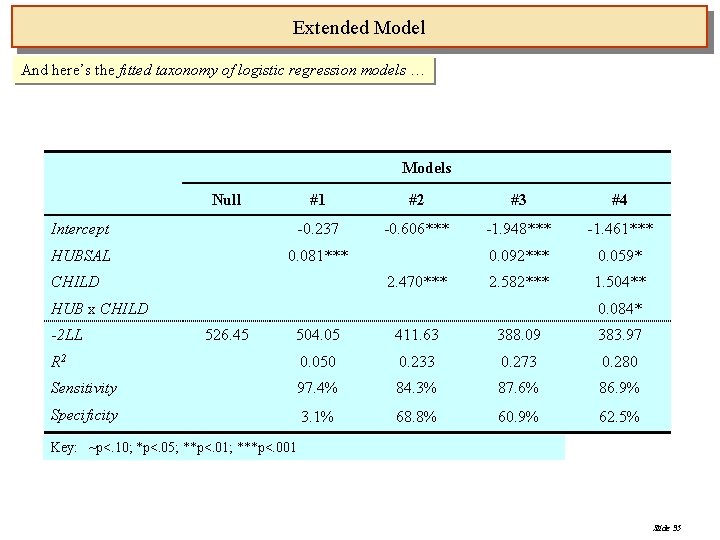
Extended Model And here’s the fitted taxonomy of logistic regression models … Models Null #1 #2 #3 #4 Intercept -0. 237 -0. 606*** -1. 948*** -1. 461*** HUBSAL 0. 081*** 0. 092*** 0. 059* 2. 582*** 1. 504** CHILD 2. 470*** HUB x CHILD -2 LL 0. 084* 526. 45 504. 05 411. 63 388. 09 383. 97 R 2 0. 050 0. 233 0. 273 0. 280 Sensitivity 97. 4% 84. 3% 87. 6% 86. 9% Specificity 3. 1% 68. 8% 60. 9% 62. 5% Key: ~p<. 10; *p<. 05; **p<. 01; ***p<. 001 Slide 35

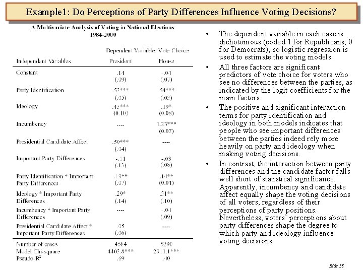
Example 1: Do Perceptions of Party Differences Influence Voting Decisions? • • The dependent variable in each case is dichotomous (coded 1 for Republicans, 0 for Democrats), so logistic regression is used to estimate the voting models. All three factors are significant predictors of vote choice for voters who see no differences between the parties, as indicated by the logit coefficients for the main factors. The positive and significant interaction terms for party identification and ideology in both models indicates that people who see important differences between the parties indeed rely more heavily on party and ideology when making voting decisions. In contrast, the interaction between party differences and the candidate factor falls well short of statistical significance. Apparently, incumbency and candidate affect equally shape the voting decisions of all voters, regardless of their perceptions of party positions. Nevertheless, voters’ perceptions about party differences shape the degree to which party and ideology influence voting decisions. Slide 36

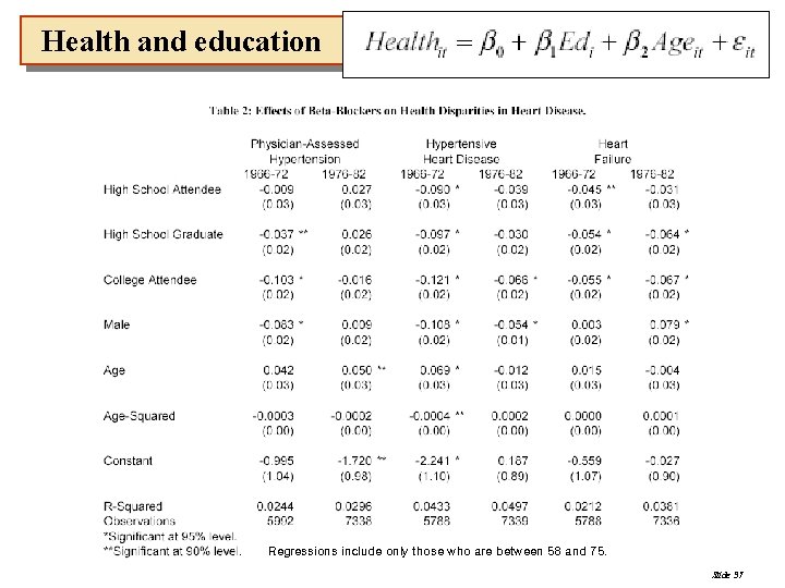
Health and education Regressions include only those who are between 58 and 75. Slide 37

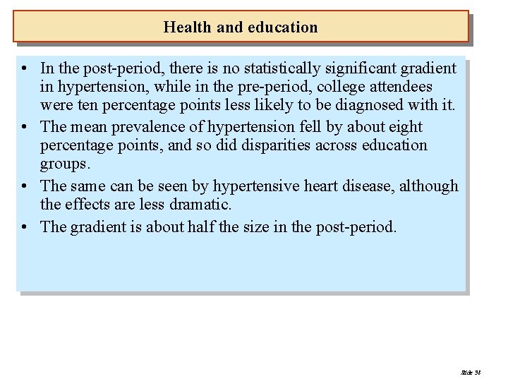
Health and education • In the post-period, there is no statistically significant gradient in hypertension, while in the pre-period, college attendees were ten percentage points less likely to be diagnosed with it. • The mean prevalence of hypertension fell by about eight percentage points, and so did disparities across education groups. • The same can be seen by hypertensive heart disease, although the effects are less dramatic. • The gradient is about half the size in the post-period. Slide 38

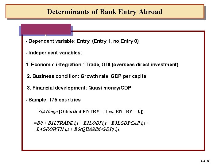
Determinants of Bank Entry Abroad - Dependent variable: Entry (Entry 1, no Entry 0) - Independent variables: 1. Economic integration : Trade, ODI (overseas direct investment) 2. Business condition: Growth rate, GDP per capita 3. Financial development: Quasi money/GDP - Sample: 175 countries Yi, t (Loge [Odds that ENTRY = 1 vs. ENTRY = 0]) =B 0 + B 1 LTRADE i, t + B 2 LODI i, t + B 3 LGDPCAP i, t + B 4 GROWTH i, t + B 5(QUASIM/GDP) i, t Slide 39

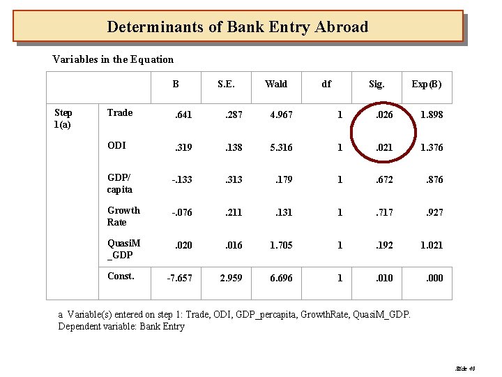
Determinants of Bank Entry Abroad Variables in the Equation B Step 1(a) S. E. Wald df Sig. Exp(B) Trade . 641 . 287 4. 967 1 . 026 1. 898 ODI . 319 . 138 5. 316 1 . 021 1. 376 GDP/ capita -. 133 . 313 . 179 1 . 672 . 876 Growth Rate -. 076 . 211 . 131 1 . 717 . 927 Quasi. M _GDP . 020 . 016 1. 705 1 . 192 1. 021 -7. 657 2. 959 6. 696 1 . 010 . 000 Const. a Variable(s) entered on step 1: Trade, ODI, GDP_percapita, Growth. Rate, Quasi. M_GDP. Dependent variable: Bank Entry Slide 40

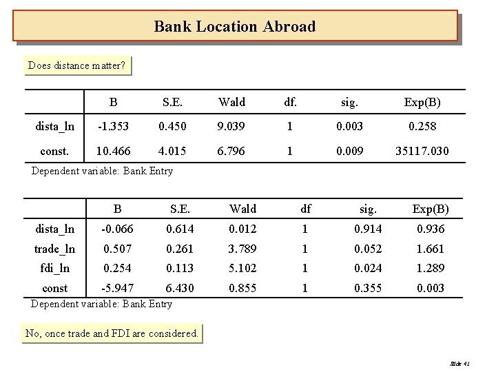
Bank Location Abroad Does distance matter? B S. E. Wald df. sig. Exp(B) dista_ln -1. 353 0. 450 9. 039 1 0. 003 0. 258 const. 10. 466 4. 015 6. 796 1 0. 009 35117. 030 Dependent variable: Bank Entry B S. E. Wald df sig. Exp(B) dista_ln -0. 066 0. 614 0. 012 1 0. 914 0. 936 trade_ln 0. 507 0. 261 3. 789 1 0. 052 1. 661 fdi_ln 0. 254 0. 113 5. 102 1 0. 024 1. 289 const -5. 947 6. 430 0. 855 1 0. 355 0. 003 Dependent variable: Bank Entry No, once trade and FDI are considered. Slide 41

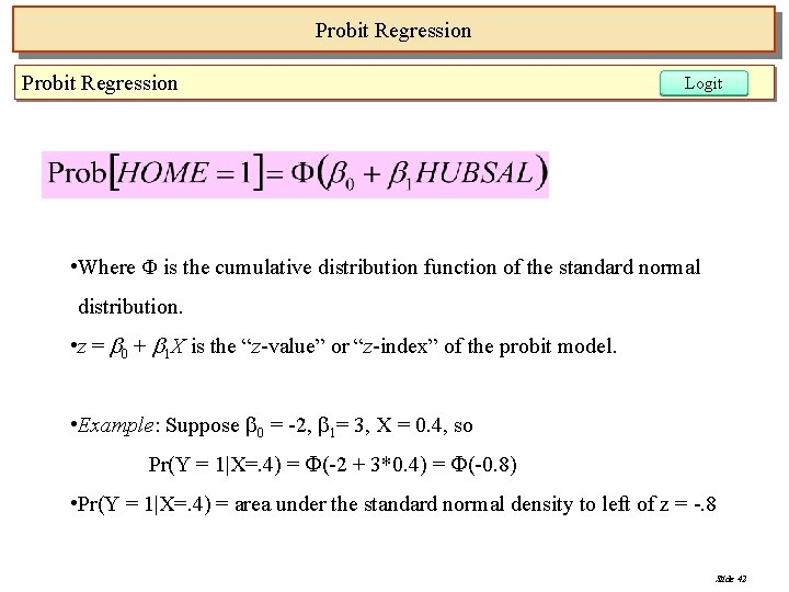
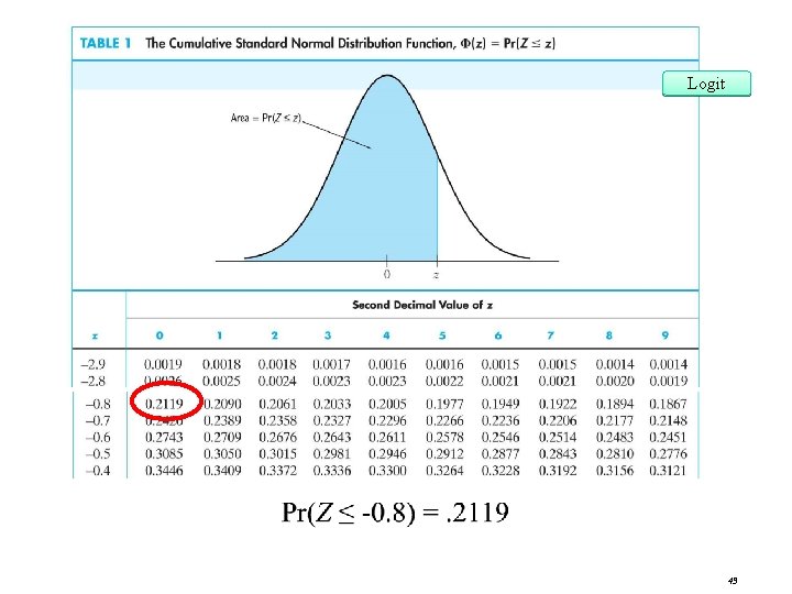
Probit Regression Logit • Where Φ is the cumulative distribution function of the standard normal distribution. • z = 0 + 1 X is the “z-value” or “z-index” of the probit model. • Example: Suppose 0 = -2, 1= 3, X = 0. 4, so Pr(Y = 1|X=. 4) = (-2 + 3*0. 4) = (-0. 8) • Pr(Y = 1|X=. 4) = area under the standard normal density to left of z = -. 8 Slide 42

Logit 43

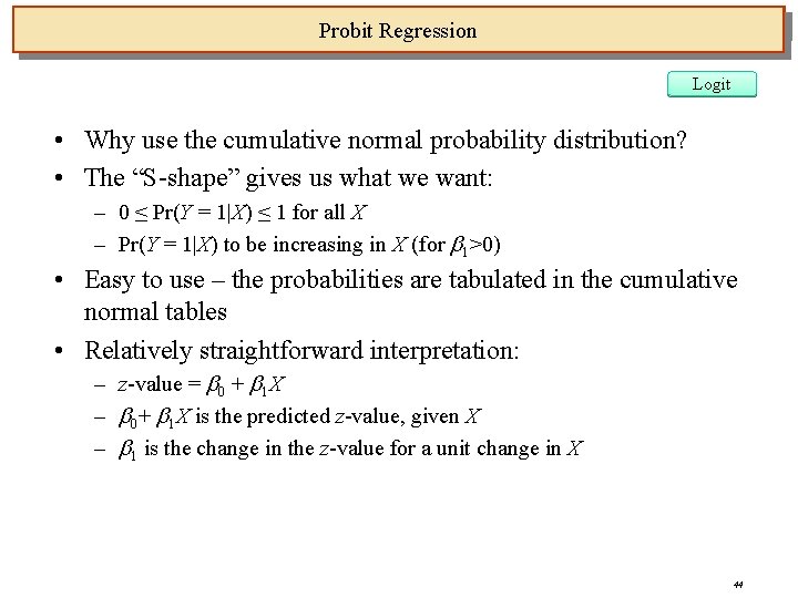
Probit Regression Logit • Why use the cumulative normal probability distribution? • The “S-shape” gives us what we want: – 0 ≤ Pr(Y = 1|X) ≤ 1 for all X – Pr(Y = 1|X) to be increasing in X (for 1>0) • Easy to use – the probabilities are tabulated in the cumulative normal tables • Relatively straightforward interpretation: – z-value = 0 + 1 X – 0+ 1 X is the predicted z-value, given X – 1 is the change in the z-value for a unit change in X 44