Regression Analysis overview Regression analysis is the idea

Regression Analysis (overview) Regression analysis is the idea of • analyzing a set of sample data and • establishing a relationship between two variables and • explaining how one variable is dependent upon the other • using this dependency to explain the population or for the prediction of future data (life expectancy example: see Excel)

Regression Analysis (overview cont’d) Regression analysis is the idea of • analyzing a set of sample data and • establishing a relationship between two variables and • explaining how one variable is dependent upon the other • using this dependency to explain the population or for the prediction of future data Regarding the second item, we will study linear relationships. Regarding the third item, we can extend the analysis to show one variable is dependent upon many variables.

Linear relationships When two variables have a linear relationship, we call them X = independent variable (horizontal axis) Y = dependent variable (vertical axis) and describe the relationship as Y = a + b*X where a = intercept b = slope (see Excel-life expectancy) For example, X = Year Y = Male Life Expectancy a = -445. 95 b = 0. 2608

Linear Relationships (cont’d) Y = a + b*X, where a is the intercept and b is the slope The intercept a is the value of Y when X = 0, or the place on the vertical axis where the line crosses The slope b describes the pitch or slope of the line If b > 0, the line goes up from left to right; the variables have a positive relationship; “when X goes up, Y goes up” If b < 0, the line goes down from left to right; the variables have a negative relationship; “when X goes up, Y goes down” In regression, we will take two variables X and Y and determine the a and b that best describe the relationship between X and Y Our starting assumption is that Y is dependent on X

Doing Regression Analysis 1. Do a scatter diagram on the relevant data 2. Add a trendline, displaying the equation as well as R 2 3. Do the full regression analysis using Excel’s Tools > Data Analysis > Regression command, saving and plotting the residuals 4. Examine the residuals for individual information (and other trends)

Method of Least Squares Think about trying to fit the line Y = a + b*X to the data, for whatever values of a and b that you wish How good is the fit? The smaller the residuals / errors the better X Y actual Y predicted Residual 2 2 3 5 + 2*2 = 9 3 - 9 = -6 36 5 -1 5 + 2*5 = 15 -1 - 15 = -16 256 36 + 256 = 292 SSE = Sum of Squares Error = amount of variability “not explained” by line

Method of Least Squares (cont’d) The main goal of the least squares method is to choose a and b so that SSE is minimized

Method of Least Squares (cont’d) SSR = Sum of Squares due to Regression = amount of variability explained by the regression SST = SSR + SSE total variability = explained variability + unexplained variability R 2 = SSR / SST = percentage of variability in Y that is explained by X = “sample coefficient of determination” Because of the above equations and the definition of SST, minimizing SSE is the same as maximizing SSR and / or R 2 is not the best measure of fit

Method of Least Squares (cont’d) A better measure of fit is… Standard error of the estimation, denoted by Se Se is the standard deviation of the residuals about their mean The smaller SSE, the smaller Se

Practical Trends with R 2 and Se When working with regression, you will often have to compare two separate regressions and try to determine which is a better model. In this case, look for higher R 2 and lower Se

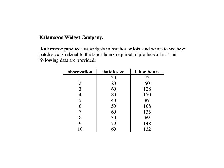
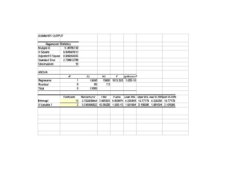
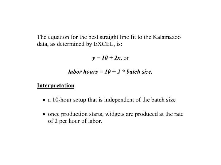
See “KLMZOO” Spreadsheet

Take a Look at “regression example” In the Regression Excel File

Point Estimates From Regression

More about the Regression Output When you use the least squares method to perform a regression analysis, here is a very important fact: the mean of all residuals equals 0

More on the Regression Output (cont’d) In a regression, what does a slope coefficient of 0 mean? It means that X has no effect on Y at all The regression output gives a 95% confidence interval for the slope coefficient: • if 0 is outside the interval, then we are confident that the slope is not 0 • if 0 is inside the interval, then the slope may be 0 P-value (or Prob-value) is “the probability that 0 is the real slope coefficient” Generally speaking, to make inferences from the regression, you want the P-value to be small (less than 0. 05)

A good regression model has… • A high R 2 value • A low Se value • Slope coefficient which is not likely to equal 0 – 0 is outside the 95% confidence interval – P-value is less than 0. 05 So then what makes a bad model?

A bad regression model has… • Residuals that are not very well distributed – overall • residual histogram should look normal – for each section of values of X • residual plot should not have any strong patterns • e. g. , mean of section’s residuals should equal 0 (like entire model) – for each subcollection of non-biased sample data • e. g. , mean of subcollection’s residuals should equal 0 (like entire model) – in other words, we want no systematic misprediction • The linear idea just doesn’t fit the situation – Do you have strong reason to believe that Y and X are not related by a line?

A bad regression model has… (cont’d) • Is the distribution of residuals non-normal? • Is the linear model inappropriate? When one of these is “yes” and the difference from the ideal model is striking, then linear regression is probably not a good idea When one of these is “yes” but the difference from the ideal model is moderate, then maybe the linear regression can be improved… (see Excel, temperature, air passenger miles)

Excel Temperature Model: Examining Residuals Sum/Avg of subcollections should be close to zero----use pivot table & grouping to examine Residuals should be normally distributed: use pivot table/chart to create histogram of residuals

Air Passenger Miles Model Does the histogram of residuals look like a normal distribution? What about the averages over subcollections of residuals?

Multiple Linear Regression Multiple linear regression is very similar to simple linear regression except that the dependent variable Y is described by m independent variables X 1, …, Xm Y = a + b 1*X 1 + … + bm*Xm (see Excel, artsy_regression. xls)

Multiple Linear Regression (cont’d) Y = a + b 1 X 1 + … + bm. Xm • Intercept a is the same • Slope bi is the change in Y given a unit change in Xi while holding all other variables constant • SST, SSE, SSR, and R 2 are the same • Se is the same except Se = sqrt( SSE / (n - m - 1) ) • Slope coefficient C. I. s (one for each Xi) are the same • P-values (one for each Xi) are the same (see Excel, artsy_regression. xls)

Dummy Variables Dummy variables are variables that only take on the values 0 or 1 can be used as a tool to put variables that do not have a natural numerical interpretation into a regression For example, sex variable is 0 for female, 1 for male For example, dummy variables can also be used to fix the problem we saw with GRADE in the Artsy example….

Dummy Variables (cont’d) Artsy example: introduce a variable Gk for each grade, 1 if in grade, 0 if not Grade / G 1 G 2 G 3 G 4 Variable G 5 G 6 G 7 G 8 Grade 1 1 0 0 0 0 Grade 2 0 1 0 0 0 Grade 3 0 0 1 0 0 0 Grade 4 0 0 0 1 0 0 Grade 5 0 0 1 0 0 0 Grade 6 0 0 0 1 0 0 Grade 7 0 0 0 1 0 Grade 8 0 0 0 0 1

Dummy Variables (cont’d) You must choose a “base case”; in this case Grade 1 is a good base case, which means we should delete the variable G 1 Grade / G 2 G 3 G 4 Variable G 5 G 6 G 7 G 8 Grade 1 0 0 0 0 Grade 2 1 0 0 0 Grade 3 0 1 0 0 0 Grade 4 0 0 1 0 0 Grade 5 0 0 0 1 0 0 0 Grade 6 0 0 1 0 0 Grade 7 0 0 0 1 0 Grade 8 0 0 0 1

Dummy Variables (cont’d) • Add these variables to your regression in place of GRADE • Rerun regression • New regression eliminates earlier problems (see Excel, artsy_regression. xls)

Why not add ALL dummy variables? Doing so creates Linear Dependency problems See Salary Data Spreadsheet: What happens when you include all the dummy variables?

A Basic Technique for Multiple Linear Regression analysis is all about trying to determine what variables have an effect on a single variable In other words, you are trying to describe Y in terms of X 1, …, Xm Some of the variables may not have a significant effect (which corresponds to a high P-value for the corresponding slope coefficient) Efficiency: Adding in variables is okay, but remove the ones that don’t have a significant effect on Y

Rough Flow Chart for Regression Do regression residuals okay but not great? high P-value? Remove variables residuals very bad or you feel “linear” is not right? Consider alternatives to linear regression Examine residuals for evidence of systematic misprediction evidence found? repeat Consider how to improve the model (e. g. , add variables) When comparing different models also take into account changes in R 2 and Se