Regression Analysis l Scatter Plots l Correlation r

Regression Analysis l. Scatter Plots l. Correlation (r) and r 2, Hypothesis Test for r l. Correlation Vs. Causation l. Residuals and the regression line l. Prediction Intervals

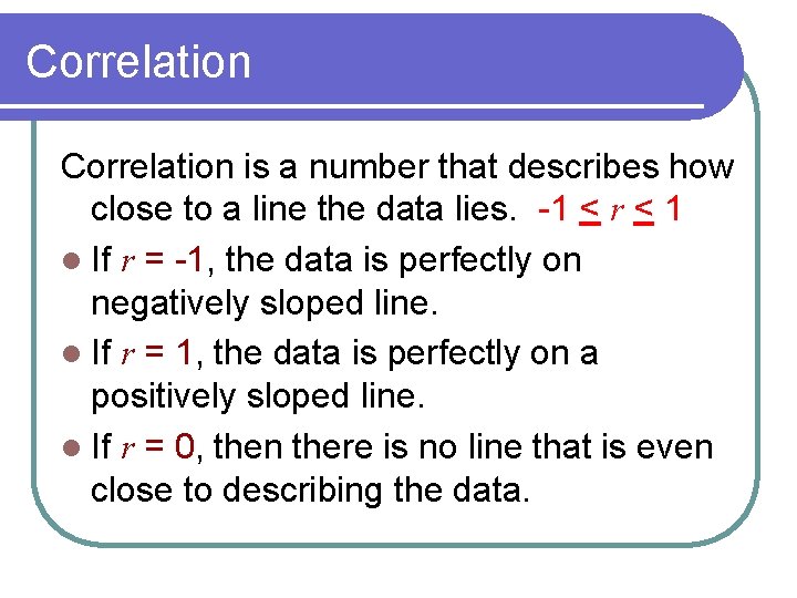
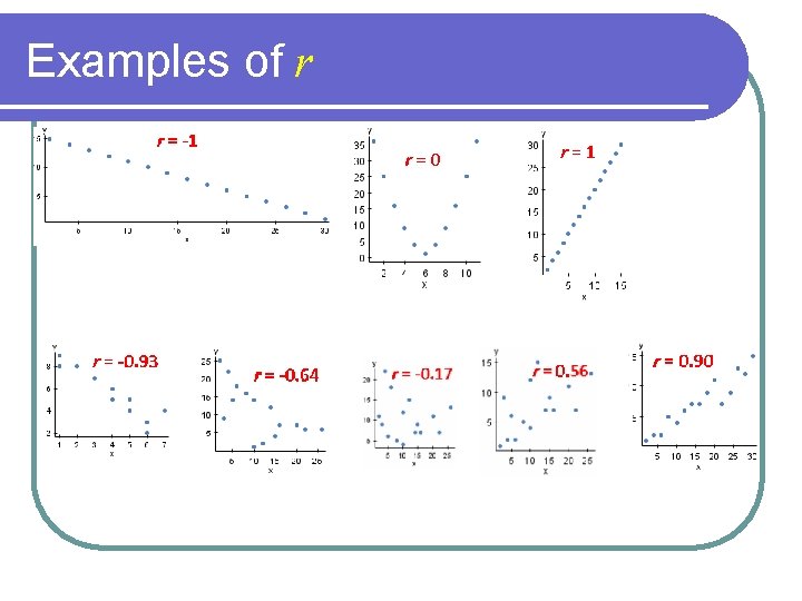
Correlation is a number that describes how close to a line the data lies. -1 < r < 1 l If r = -1, the data is perfectly on negatively sloped line. l If r = 1, the data is perfectly on a positively sloped line. l If r = 0, then there is no line that is even close to describing the data.

Examples of r

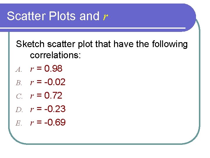
Scatter Plots and r Sketch scatter plot that have the following correlations: A. r = 0. 98 B. r = -0. 02 C. r = 0. 72 D. r = -0. 23 E. r = -0. 69

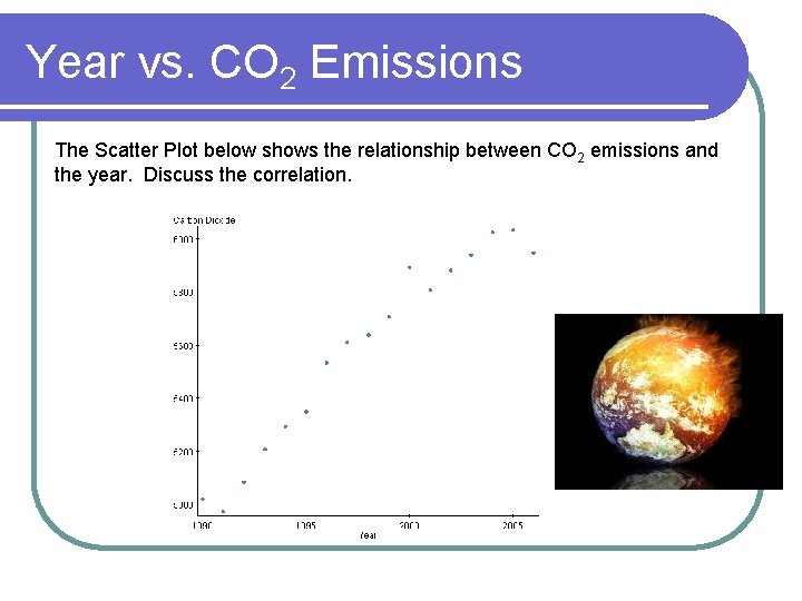
Year vs. CO 2 Emissions The Scatter Plot below shows the relationship between CO 2 emissions and the year. Discuss the correlation.

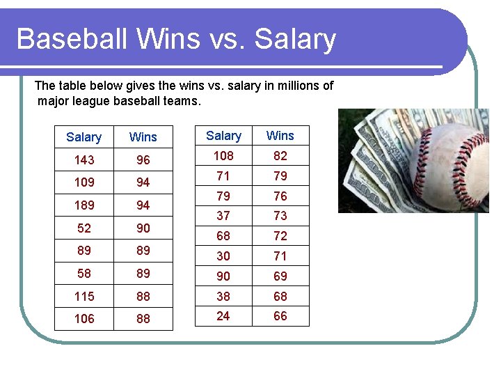
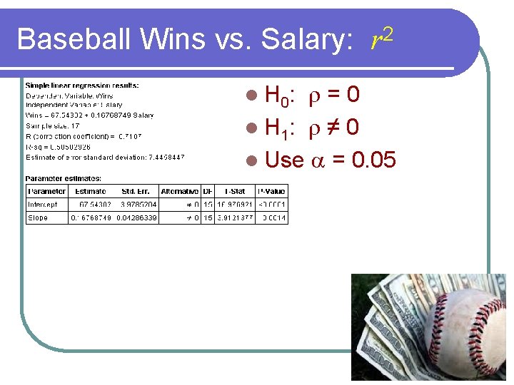
Baseball Wins vs. Salary The table below gives the wins vs. salary in millions of major league baseball teams. Salary Wins 143 96 108 82 109 94 71 79 189 94 79 76 52 90 37 73 68 72 89 89 30 71 58 89 90 69 115 88 38 68 106 88 24 66

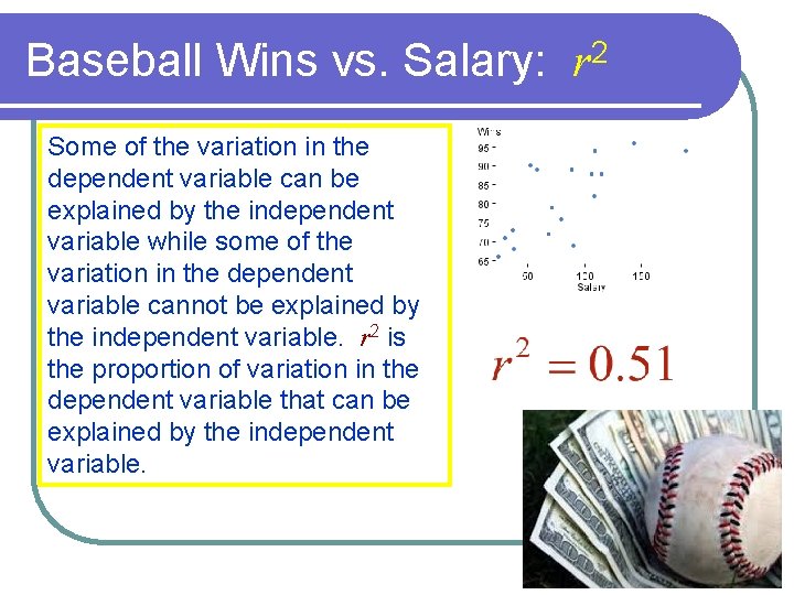
Baseball Wins vs. Salary: r 2 Some of the variation in the dependent variable can be explained by the independent variable while some of the variation in the dependent variable cannot be explained by the independent variable. r 2 is the proportion of variation in the dependent variable that can be explained by the independent variable.

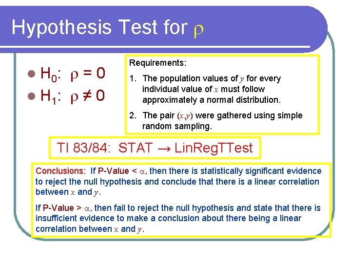
Hypothesis Test for r r=0 l H 1: r ≠ 0 l H 0: Requirements: 1. The population values of y for every individual value of x must follow approximately a normal distribution. 2. The pair (x, y) were gathered using simple random sampling. TI 83/84: STAT → Lin. Reg. TTest Conclusions: If P-Value < a, then there is statistically significant evidence to reject the null hypothesis and conclude that there is a linear correlation between x and y. If P-Value > a, then fail to reject the null hypothesis and state that there is insufficient evidence to make a conclusion about there being a linear correlation between x and y.

Baseball Wins vs. Salary: r 2 r=0 l H 1: r ≠ 0 l Use a = 0. 05 l H 0:

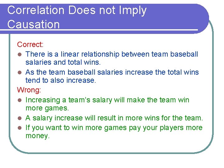
Correlation Does not Imply Causation Correct: l There is a linear relationship between team baseball salaries and total wins. l As the team baseball salaries increase the total wins tend to also increase. Wrong: l Increasing a team’s salary will make the team win more games. l A salary increase will result in more wins for the team. l If you want to win more games pay your players more money.

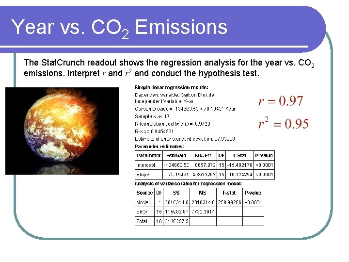
Year vs. CO 2 Emissions The Stat. Crunch readout shows the regression analysis for the year vs. CO 2 emissions. Interpret r and r 2 and conduct the hypothesis test.

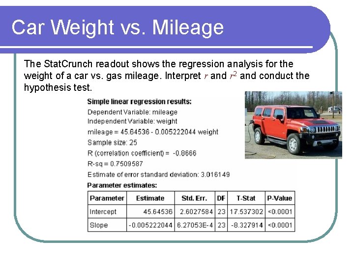
Car Weight vs. Mileage The Stat. Crunch readout shows the regression analysis for the weight of a car vs. gas mileage. Interpret r and r 2 and conduct the hypothesis test.

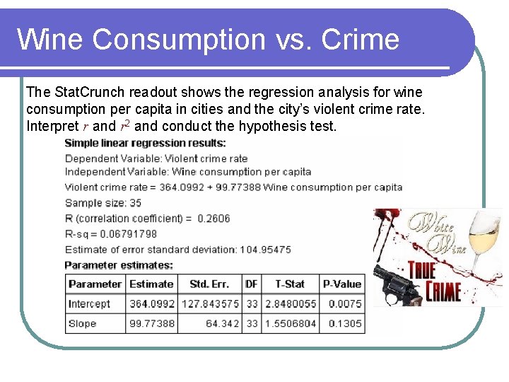
Wine Consumption vs. Crime The Stat. Crunch readout shows the regression analysis for wine consumption per capita in cities and the city’s violent crime rate. Interpret r and r 2 and conduct the hypothesis test.

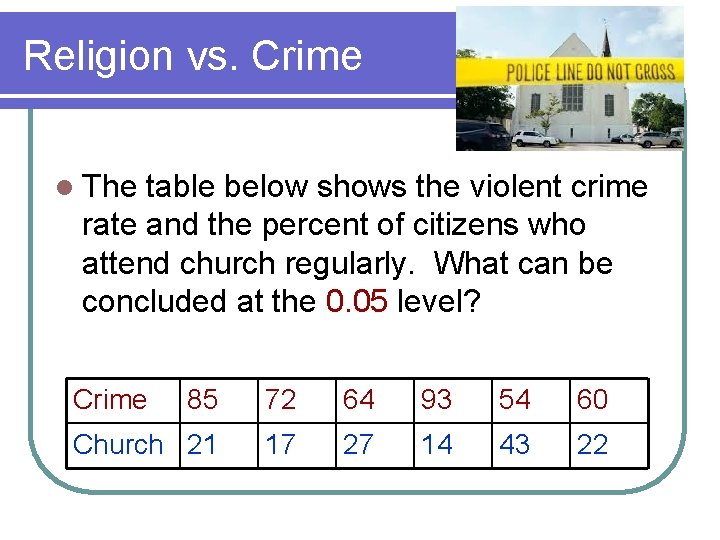
Religion vs. Crime l The table below shows the violent crime rate and the percent of citizens who attend church regularly. What can be concluded at the 0. 05 level? Crime 85 72 64 93 54 60 Church 21 17 27 14 43 22

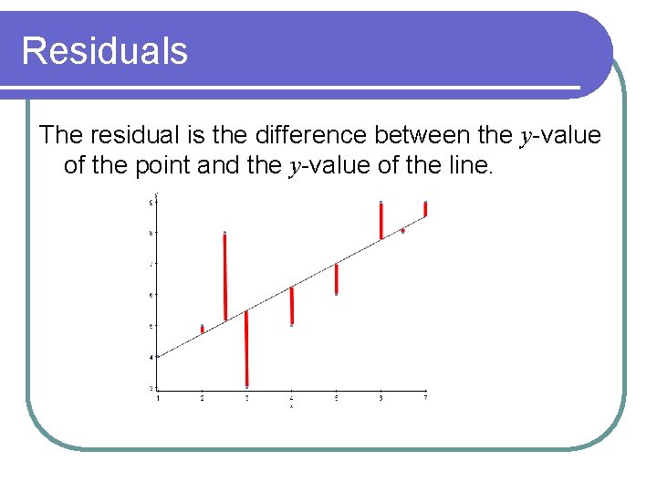
Residuals The residual is the difference between the y-value of the point and the y-value of the line.

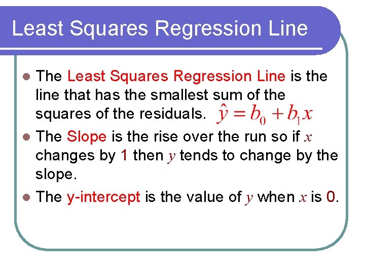
Least Squares Regression Line The Least Squares Regression Line is the line that has the smallest sum of the squares of the residuals. l The Slope is the rise over the run so if x changes by 1 then y tends to change by the slope. l The y-intercept is the value of y when x is 0. l

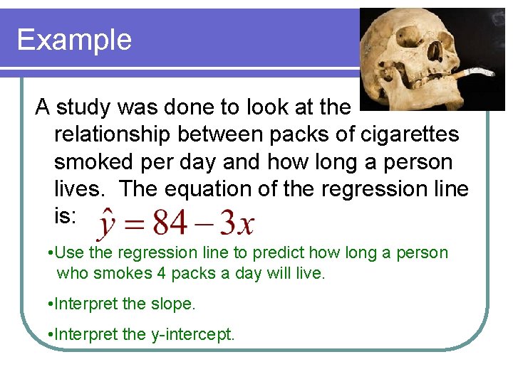
Example A study was done to look at the relationship between packs of cigarettes smoked per day and how long a person lives. The equation of the regression line is: • Use the regression line to predict how long a person who smokes 4 packs a day will live. • Interpret the slope. • Interpret the y-intercept.

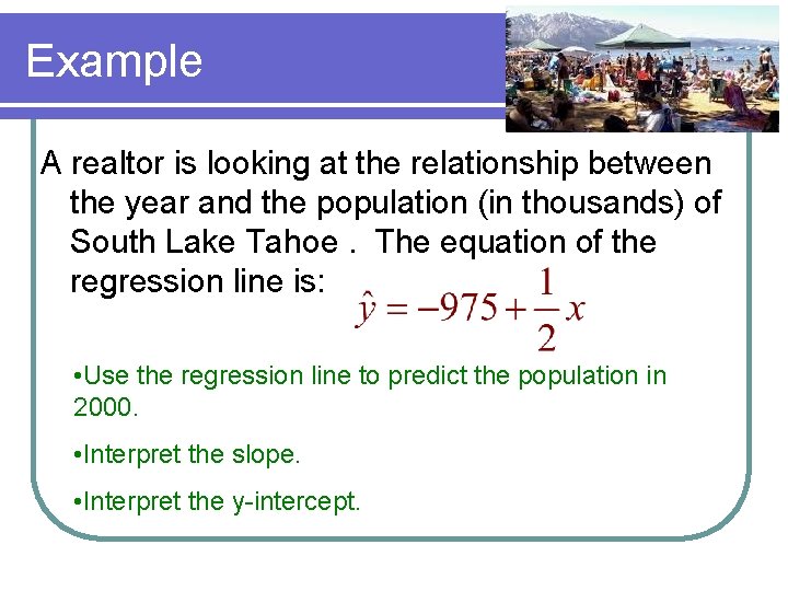
Example A realtor is looking at the relationship between the year and the population (in thousands) of South Lake Tahoe. The equation of the regression line is: • Use the regression line to predict the population in 2000. • Interpret the slope. • Interpret the y-intercept.

Prediction Interval We can use the regression line to make a prediction for y given an x. This is just a prediction and has error. We can form a confidence interval for the this y given x. If r 2 is large, then it is useful to use the value of x to predict y. Otherwise it is not useful.

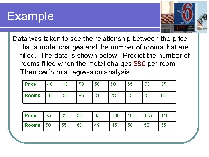
Example Data was taken to see the relationship between the price that a motel charges and the number of rooms that are filled. The data is shown below. Predict the number of rooms filled when the motel charges $80 per room. Then perform a regression analysis. Price 40 40 50 50 60 65 70 75 Rooms 92 80 85 81 78 75 80 65 Price 85 85 90 95 100 105 110 Rooms 50 55 60 49 45 50 52 35

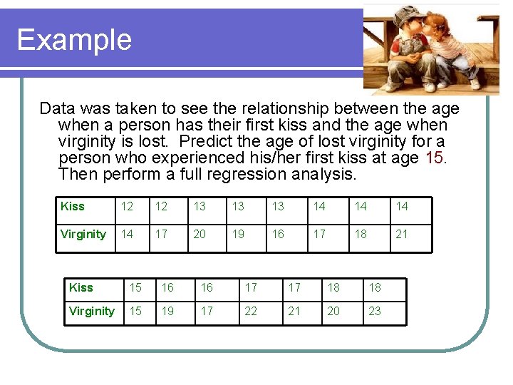
Example Data was taken to see the relationship between the age when a person has their first kiss and the age when virginity is lost. Predict the age of lost virginity for a person who experienced his/her first kiss at age 15. Then perform a full regression analysis. Kiss 12 12 13 13 13 14 14 14 Virginity 14 17 20 19 16 17 18 21 Kiss 15 16 16 17 17 18 18 Virginity 15 19 17 22 21 20 23