Regression Analysis in Theory and Practice DONT WRITE


 0 3 1 y (sen")
")
 * 4 a = 26 –")


- Slides: 21
Regression Analysis in Theory and Practice
DON’T WRITE THE FORMULAS AHEAD!!!
REGRESSION ANALYSIS Formula for simple regression where is the predicted value of Y on the regression line. Do you remember y=mx + b? Same thing!
The dependence of Y on X can be of two types: “deterministic” or “probabilistic”. The classic case of deterministic relationship is that between Fahrenheit and Celsius measure of temperature: F 0 = 32 + (9/5)C Where a, the intercept, is 320. So when C=0, degrees F=32, b beta, is the slope of the line, here (9/5) or 1. 8. C is X, degrees Celsius.
So for every on degree of change in degrees C, Fahrenheit goes up by 1. 8 degrees, starting at 32 degrees. So when C =0 F = 320 + (9/5)0 = 320 When C = 1000 F = 32 + (9/5)100=2120 Note: 1. 8 = 9/5
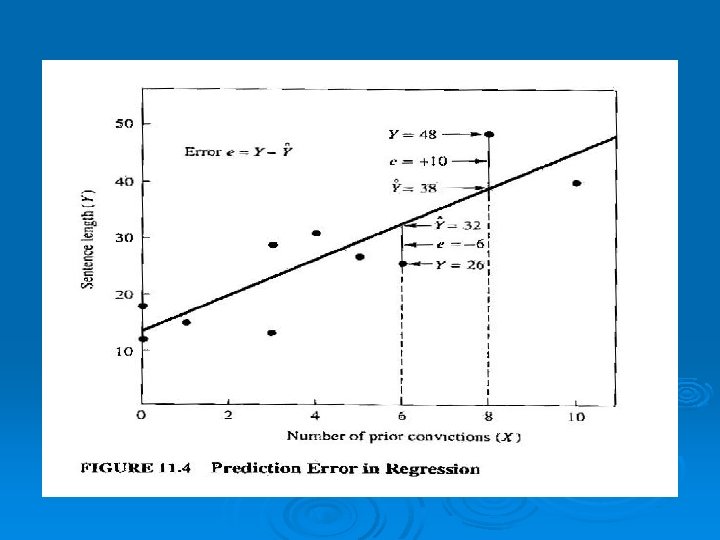
Probabilistic Regression Ø Not perfectly predictive. Ø On average, we expect a certain amount of change in Y for a certain change in X
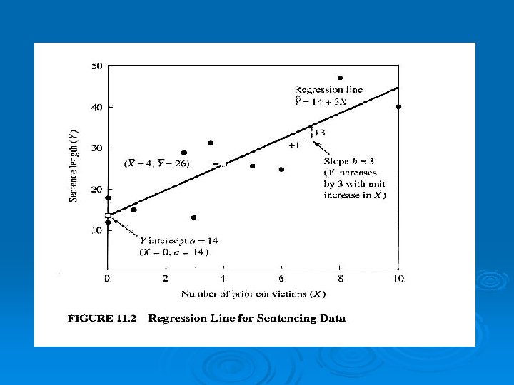
Regression Example Ø Judges are advised to give longer sentences to repeat offenders than to firsttime offenders. Does it really happen? Ø Hypothesis: In comparing criminals, those who illustrate the characteristic of having been convicted before will receive longer prison sentences than those with no prior convictions. Ø We collect data for 10 convicted criminals
Data and Formula: X=4 Y = 26 X (convctn) 0 3 1 y (sen len) 12 13 15 X–X -4 -1 -3 Y–Y -14 -13 -11 0 6 5 3 4 10 8 Σx = 40 19 26 27 29 31 40 48 Σy = 260 -4 2 1 -1 0 6 4 -7 0 1 3 5 84 88
X=4 Y = 26 Continued: X–X -4 -1 -3 Y–Y -14 -13 -11 (X-X) * (Y-Y) 56 13 33 (X-X)2 16 1 9 -4 2 1 -1 0 6 4 -7 0 1 3 5 84 88 28 0 1 -3 5 14 22 Σ = 300 16 4 1 1 0 36 16 Σ= 100 b=3
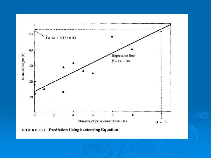
Now Calculate “A” a = 26 – (3) * 4 a = 26 – 12 a = 14 Y = 14 + 3*X
Interpret the Equation Y = 14 + 3*X Interpret 14 Interpret 3
Scatterplot
Multiple Regression - 1 Ø The mathematics of how the computer calculates regression coefficients in multiple regression is very complicated. Fortunately, there is an intuitive process that generates the correct answers and is much easier to understand. Let’s see how the computer obtained the value of. 644 for the impact of senator conservatism on the degree to which a senator voted for tax changes primarily benefitting households at, or below, the median income.
Multiple Regression - 2 Our “main equation” is: Ø Y = a 1 + b 1 X 1 + b 2 X 2 + b 3 X 3 + e 1 Ø Y = percentage support for tax changes benefitting households with incomes at, or below, the median Ø X 1 = senator conservatism Ø X 2 = senator party affiliation Ø X 3 = state median household income Ø Our goal is to estimate b 1 Ø
Multiple Regression - 3 Ø X 1 = a 2 + b 4 X 2 + b 5 X 3 + e 2 Ø In the above equation e 2 represents that portion of a senator’s conservatism than CANNOT be explained by either their party affiliation or the median family income in their state.
Multiple Regression - 4 Ø Y = a 3 + b 6 X 2 + b 7 X 3 + e 3 Ø In the above equation e 3 represents that portion of a senator’s degree of support for tax changes favorable to households with incomes at, or below, the median that CANNOT be explained by either their party affiliation or the median family income in their state.
Multiple Regression - 5 Ø e 3 = a 4 + b 8 e 2 + e 4 Ø In the above equation b 8 represents the impact of that portion of a senator’s conservatism that CANNOT be explained by party and state median income on the percentage of times the senator voted in favor of tax changes primarily benefitting households at, or below, the median income that CANNOT be explained by either their party affiliation or the median income in their state. Thus, b 8 in the above equation = b 1 in the “main equation” (i. e. , -. 644).
Maximum Likelihood Estimation