Regression Analysis Gordon Stringer UCCS 1 Regression Analysis

Regression Analysis Gordon Stringer, UCCS 1

Regression Analysis ¨ Regression Analysis: the study of the relationship between variables ¨ Regression Analysis: one of the most commonly used tools for business analysis ¨ Easy to use and applies to many situations Gordon Stringer, UCCS 2

Regression Analysis ¨ Simple Regression: single explanatory variable ¨ Multiple Regression: includes any number of explanatory variables. Gordon Stringer, UCCS 3

Regression Analysis ¨ Dependant variable: the single variable being explained/ predicted by the regression model (response variable) ¨ Independent variable: The explanatory variable(s) used to predict the dependant variable. (predictor variable) Gordon Stringer, UCCS 4

Regression Analysis ¨ Linear Regression: straight-line relationship Form: y=mx+b ¨ Non-linear: implies curved relationships, for example logarithmic relationships Gordon Stringer, UCCS 5

Data Types ¨ Cross Sectional: data gathered from the same time period ¨ Time Series: Involves data observed over equally spaced points in time. Gordon Stringer, UCCS 6

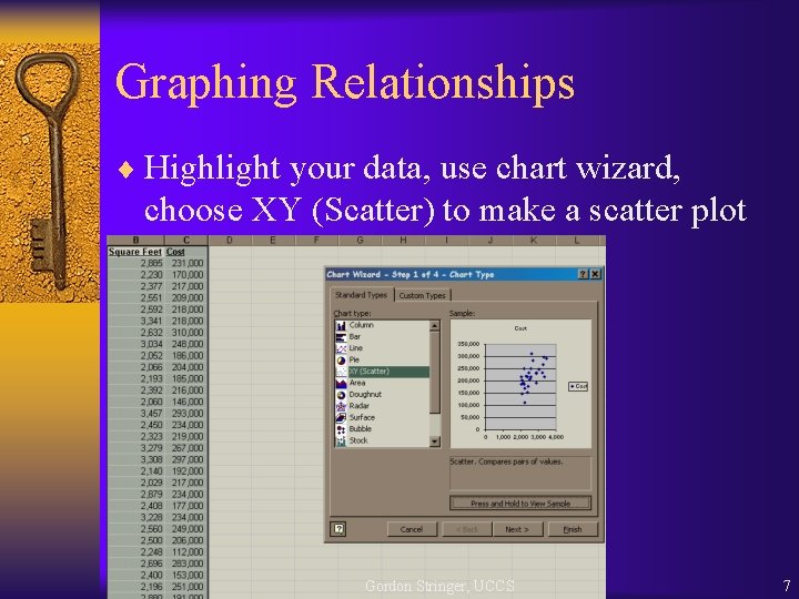
Graphing Relationships ¨ Highlight your data, use chart wizard, choose XY (Scatter) to make a scatter plot Gordon Stringer, UCCS 7

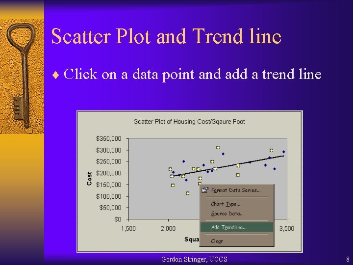
Scatter Plot and Trend line ¨ Click on a data point and add a trend line Gordon Stringer, UCCS 8

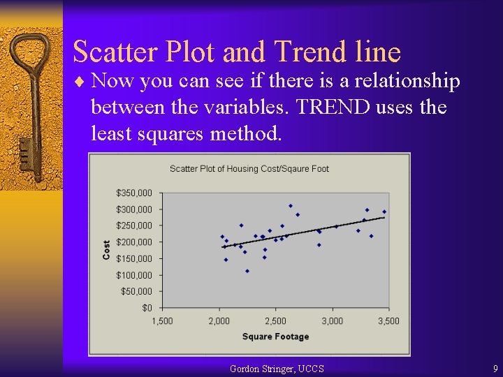
Scatter Plot and Trend line ¨ Now you can see if there is a relationship between the variables. TREND uses the least squares method. Gordon Stringer, UCCS 9

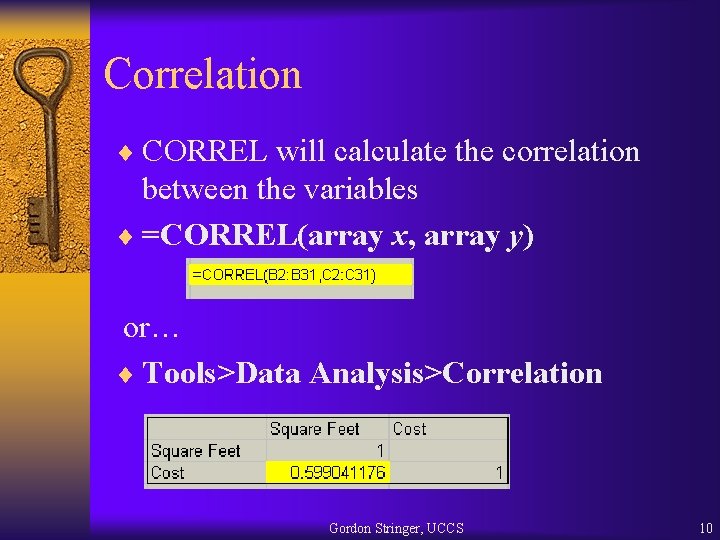
Correlation ¨ CORREL will calculate the correlation between the variables ¨ =CORREL(array x, array y) or… ¨ Tools>Data Analysis>Correlation Gordon Stringer, UCCS 10

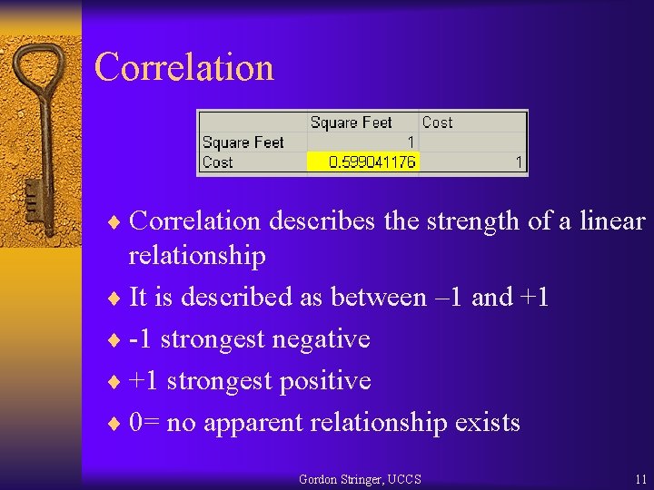
Correlation ¨ Correlation describes the strength of a linear relationship ¨ It is described as between – 1 and +1 ¨ -1 strongest negative ¨ +1 strongest positive ¨ 0= no apparent relationship exists Gordon Stringer, UCCS 11

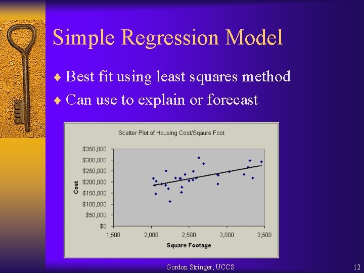
Simple Regression Model ¨ Best fit using least squares method ¨ Can use to explain or forecast Gordon Stringer, UCCS 12

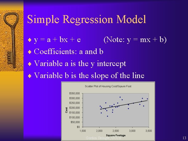
Simple Regression Model ¨ y = a + bx + e (Note: y = mx + b) ¨ Coefficients: a and b ¨ Variable a is the y intercept ¨ Variable b is the slope of the line Gordon Stringer, UCCS 13

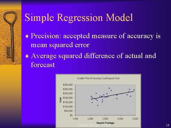
Simple Regression Model ¨ Precision: accepted measure of accuracy is mean squared error ¨ Average squared difference of actual and forecast Gordon Stringer, UCCS 14

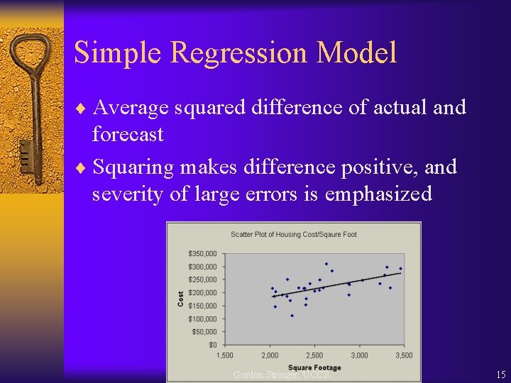
Simple Regression Model ¨ Average squared difference of actual and forecast ¨ Squaring makes difference positive, and severity of large errors is emphasized Gordon Stringer, UCCS 15

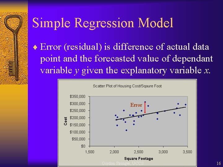
Simple Regression Model ¨ Error (residual) is difference of actual data point and the forecasted value of dependant variable y given the explanatory variable x. Error Gordon Stringer, UCCS 16

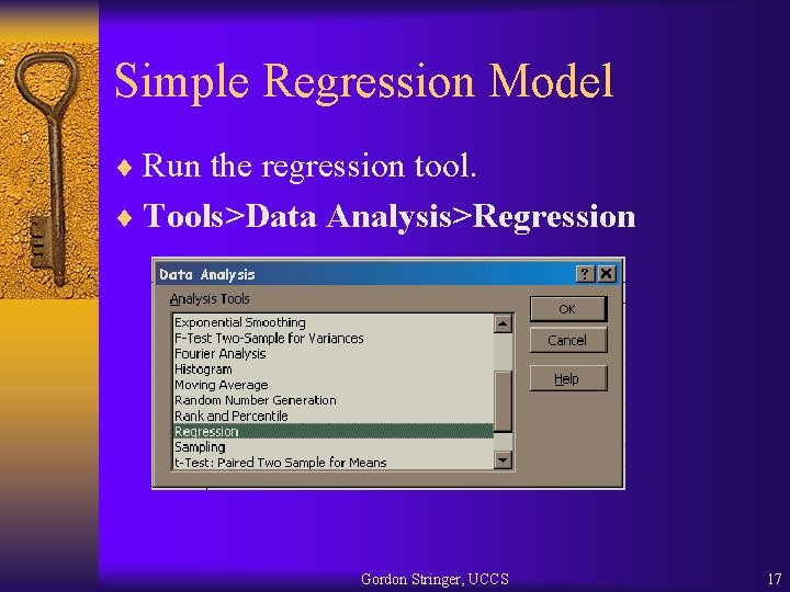
Simple Regression Model ¨ Run the regression tool. ¨ Tools>Data Analysis>Regression Gordon Stringer, UCCS 17

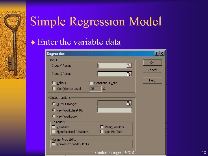
Simple Regression Model ¨ Enter the variable data Gordon Stringer, UCCS 18

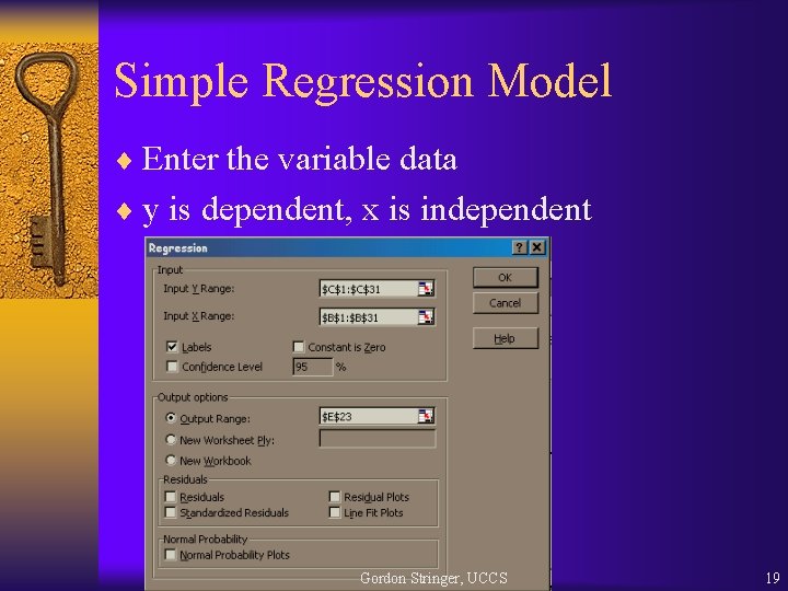
Simple Regression Model ¨ Enter the variable data ¨ y is dependent, x is independent Gordon Stringer, UCCS 19

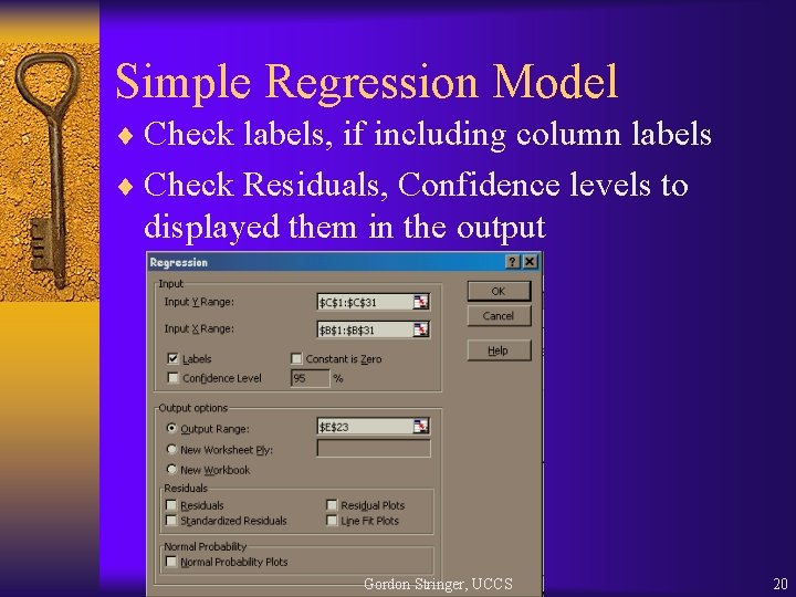
Simple Regression Model ¨ Check labels, if including column labels ¨ Check Residuals, Confidence levels to displayed them in the output Gordon Stringer, UCCS 20

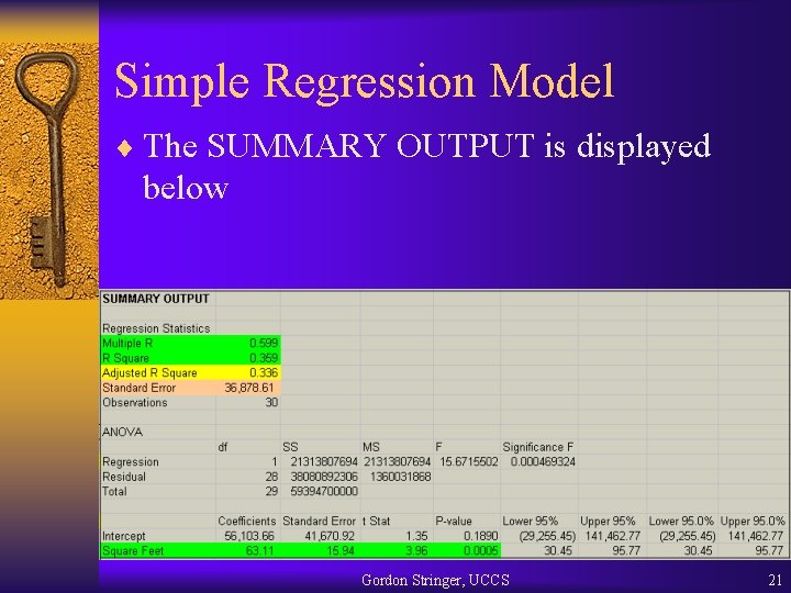
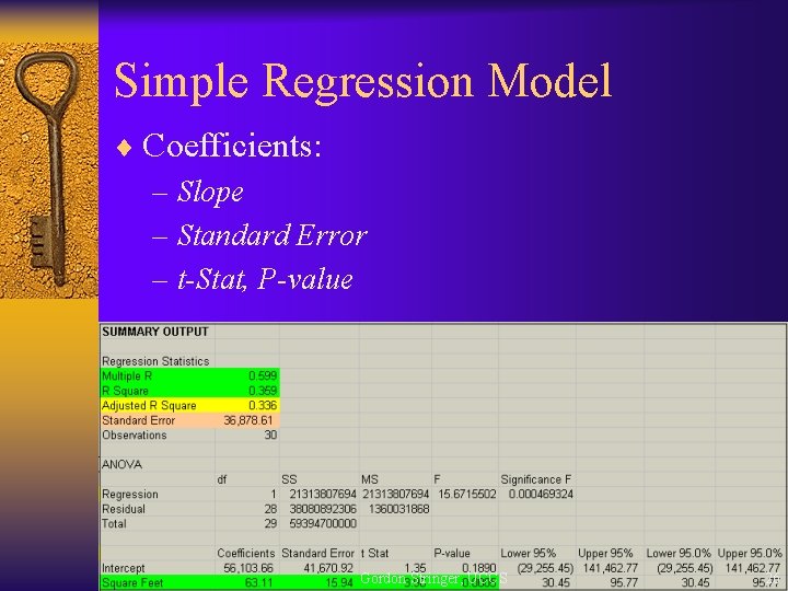
Simple Regression Model ¨ The SUMMARY OUTPUT is displayed below Gordon Stringer, UCCS 21

Simple Regression Model ¨ Multiple R is the correlation coefficient ¨ =CORREL Gordon Stringer, UCCS 22

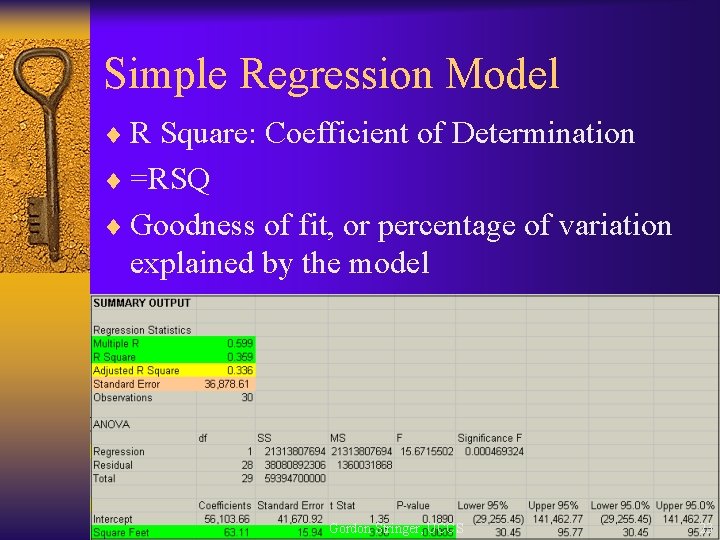
Simple Regression Model ¨ R Square: Coefficient of Determination ¨ =RSQ ¨ Goodness of fit, or percentage of variation explained by the model Gordon Stringer, UCCS 23

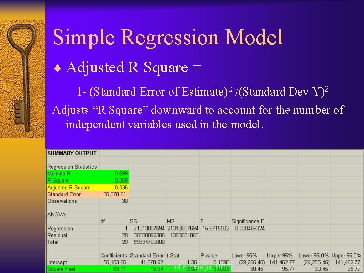
Simple Regression Model ¨ Adjusted R Square = 1 - (Standard Error of Estimate)2 /(Standard Dev Y)2 Adjusts “R Square” downward to account for the number of independent variables used in the model. Gordon Stringer, UCCS 24

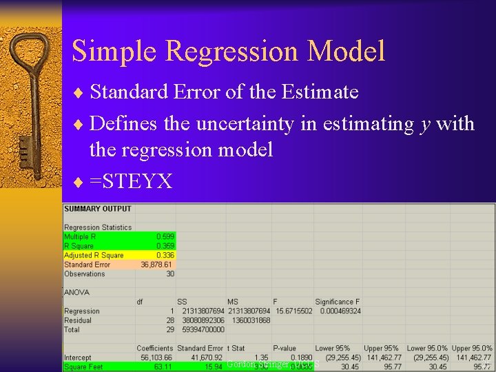
Simple Regression Model ¨ Standard Error of the Estimate ¨ Defines the uncertainty in estimating y with the regression model ¨ =STEYX Gordon Stringer, UCCS 25

Simple Regression Model ¨ Coefficients: – Slope – Standard Error – t-Stat, P-value Gordon Stringer, UCCS 26

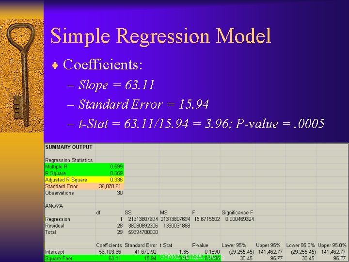
Simple Regression Model ¨ Coefficients: – Slope = 63. 11 – Standard Error = 15. 94 – t-Stat = 63. 11/15. 94 = 3. 96; P-value =. 0005 Gordon Stringer, UCCS 27

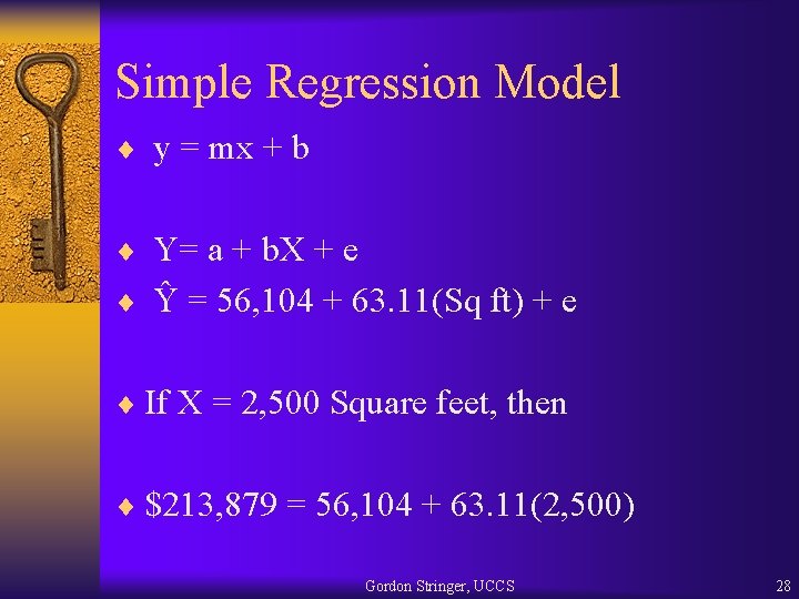
Simple Regression Model ¨ y = mx + b ¨ Y= a + b. X + e ¨ Ŷ = 56, 104 + 63. 11(Sq ft) + e ¨ If X = 2, 500 Square feet, then ¨ $213, 879 = 56, 104 + 63. 11(2, 500) Gordon Stringer, UCCS 28

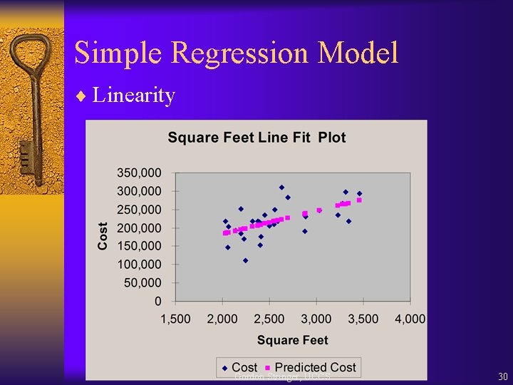
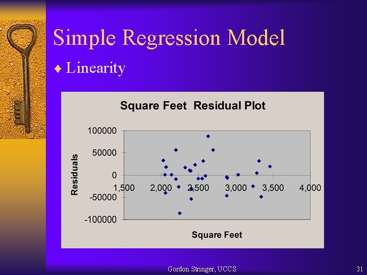
Simple Regression Model ¨ Linearity ¨ Independence ¨ Homoscedasity ¨ Normality Gordon Stringer, UCCS 29

Simple Regression Model ¨ Linearity Gordon Stringer, UCCS 30

Simple Regression Model ¨ Linearity Gordon Stringer, UCCS 31

Simple Regression Model ¨ Independence: – Errors must not correlate – Trials must be independent Gordon Stringer, UCCS 32

Simple Regression Model ¨ Homoscedasticity: – Constant variance – Scatter of errors does not change from trial to trial – Leads to misspecification of the uncertainty in the model, specifically with a forecast – Possible to underestimate the uncertainty – Try square root, logarithm, or reciprocal of y Gordon Stringer, UCCS 33

Simple Regression Model ¨ Normality: • Errors should be normally distributed • Plot histogram of residuals Gordon Stringer, UCCS 34

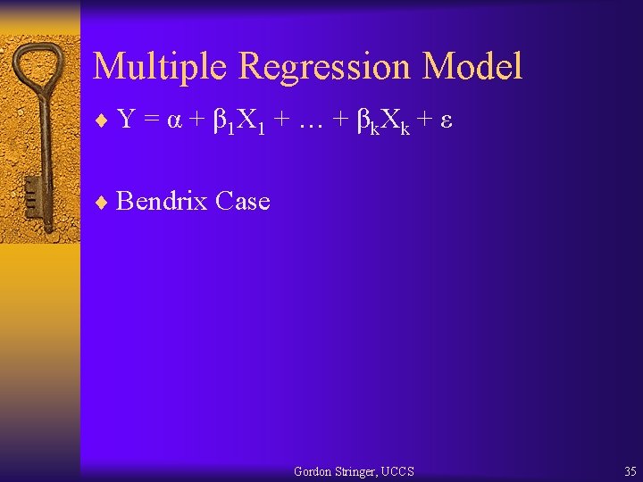
Multiple Regression Model ¨ Y = α + β 1 X 1 + … + βk. Xk + ε ¨ Bendrix Case Gordon Stringer, UCCS 35

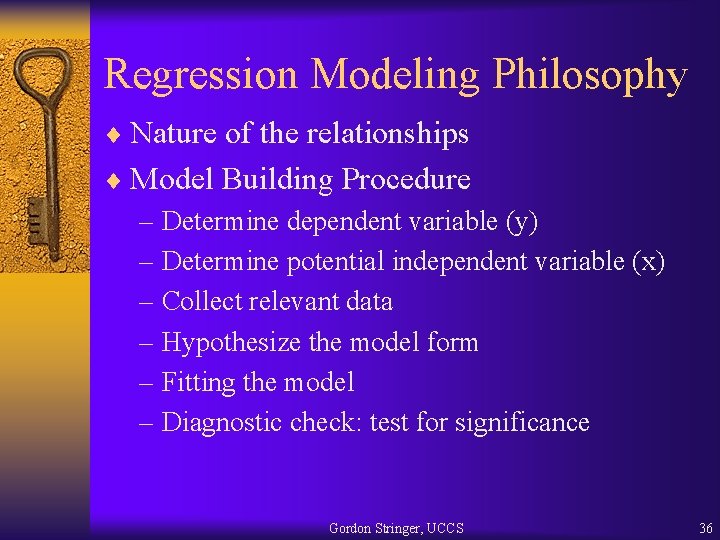
Regression Modeling Philosophy ¨ Nature of the relationships ¨ Model Building Procedure – Determine dependent variable (y) – Determine potential independent variable (x) – Collect relevant data – Hypothesize the model form – Fitting the model – Diagnostic check: test for significance Gordon Stringer, UCCS 36