Regression Analysis Fundamental Tool in Machine Learning AI

Regression Analysis Fundamental Tool in Machine Learning, AI etc. Applications: Analytical CRM, Forecasting etc. Text: Chapters 10 -11

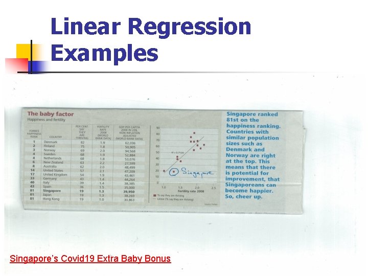
Linear Regression Examples Singapore’s Covid 19 Extra Baby Bonus

Straits Times Mon 14 Oct 2013 2019 UK elections & Currency Movements

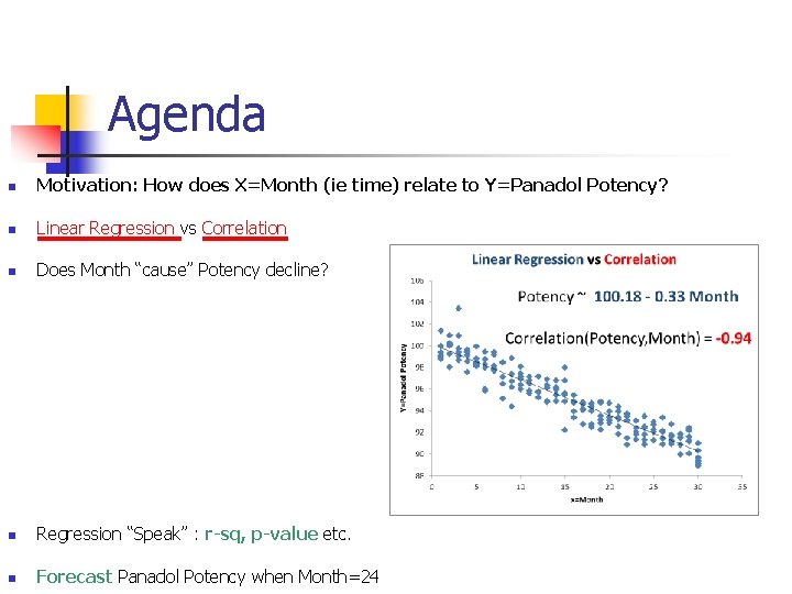
Agenda n Motivation: How does X=Month (ie time) relate to Y=Panadol Potency? n Linear Regression vs Correlation n Does Month “cause” Potency decline? n Regression “Speak” : r-sq, p-value etc. n Forecast Panadol Potency when Month=24

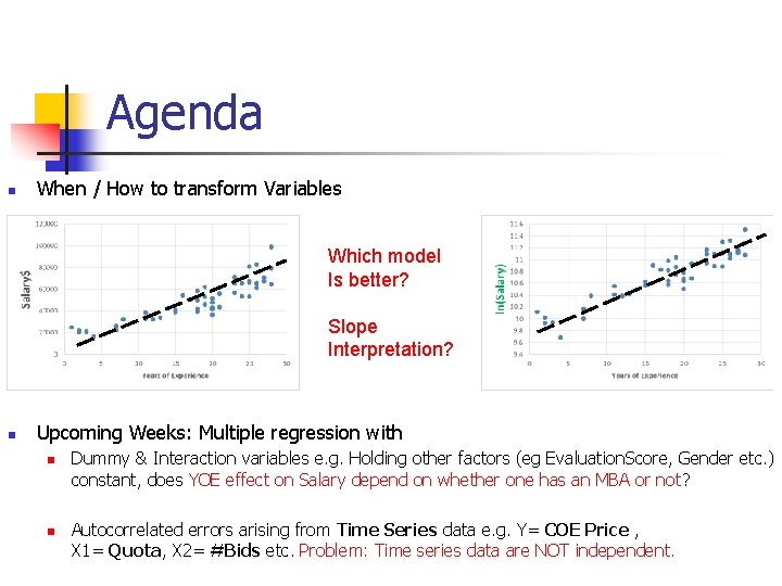
Agenda n When / How to transform Variables Which model Is better? Slope Interpretation? n Upcoming Weeks: Multiple regression with n n Dummy & Interaction variables e. g. Holding other factors (eg Evaluation. Score, Gender etc. ) constant, does YOE effect on Salary depend on whether one has an MBA or not? Autocorrelated errors arising from Time Series data e. g. Y= COE Price , X 1= Quota, X 2= #Bids etc. Problem: Time series data are NOT independent.

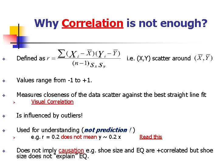
Why Correlation is not enough? v Defined as v Values range from -1 to +1. v Measures closeness of the data scatter against the best straight line fit Ø i. e. (X, Y) scatter around Visual Correlation v Is influenced by outliers! v Used for understanding (not prediction ! ) Ø v e. g. r = 0. 2 does not mean y ~ 0. 2 x Read this Does not imply causation e. g. shoe size and EQ are +correlated but shoe size does not “explain” EQ.

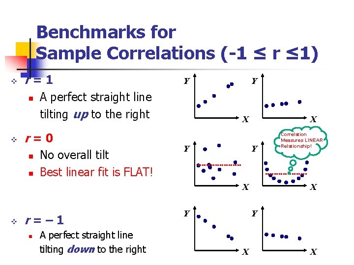
Benchmarks for Sample Correlations (-1 ≤ r ≤ 1) v r=1 n v A perfect straight line tilting up to the right r=0 n n Y No overall tilt Best linear fit is FLAT! Y X Y X v r=– 1 n A perfect straight line tilting down to the right Y Correlation Measures LINEAR Relationship! X Y X X

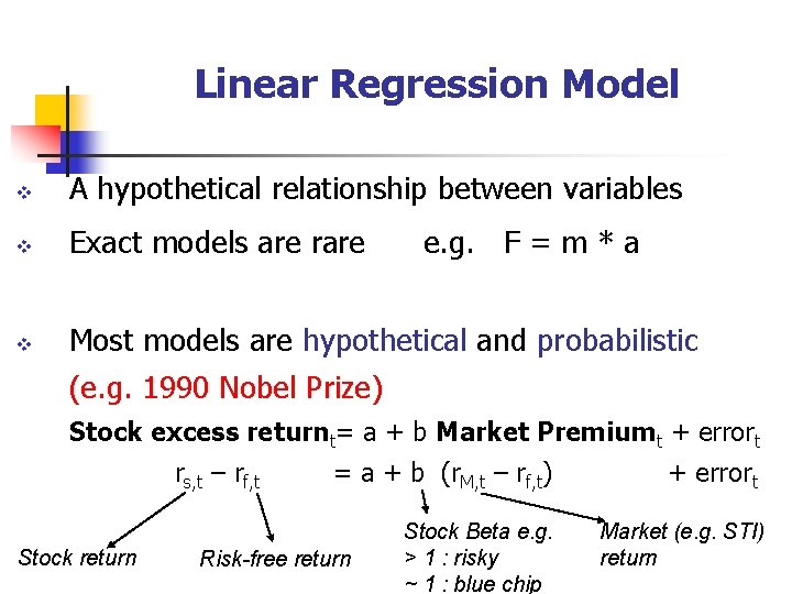
Linear Regression Model v A hypothetical relationship between variables v Exact models are rare v Most models are hypothetical and probabilistic e. g. F = m * a (e. g. 1990 Nobel Prize) Stock excess returnt= a + b Market Premiumt + errort rs, t – rf, t Stock return = a + b (r. M, t – rf, t) + errort Stock Beta e. g. > 1 : risky ~ 1 : blue chip Market (e. g. STI) return Risk-free return

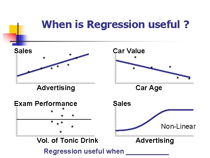
When is Regression useful ? Sales * * * * Car Value * * * Advertising Exam Performance * * ** * * Vol. of Tonic Drink Car Age * Sales Non-Linear Advertising Regression useful when ______

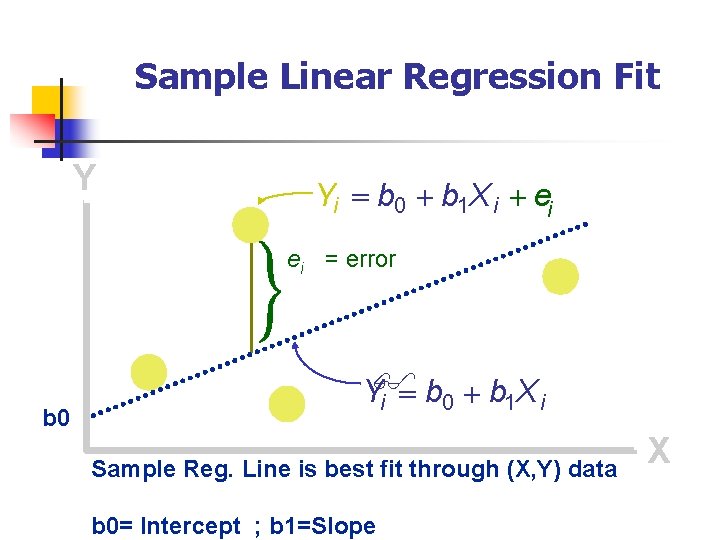
Sample Linear Regression Fit Y Yi b 0 b 1 X i ei ei = error b 0 Y i b 0 b 1 X i Sample Reg. Line is best fit through (X, Y) data b 0= Intercept ; b 1=Slope X

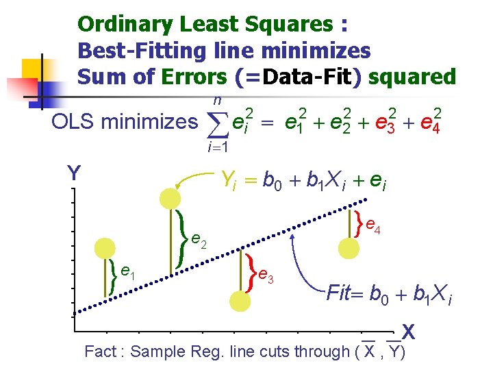
Ordinary Least Squares : Best-Fitting line minimizes Sum of Errors (=Data-Fit) squared n OLS minimizes 2 2 2 e e e i 1 2 3 4 i 1 Y Yi b 0 b 1 X i ei e 4 e 2 e 1 e 3 Fit b 0 b 1 X i X Fact : Sample Reg. line cuts through ( X , Y)

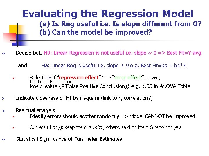
Evaluating the Regression Model (a) Is Reg useful i. e. Is slope different from 0? (b) Can the model be improved? Decide bet. H 0: Linear Regression is not useful i. e. slope ~ 0 => Best Fit=Y-avg v and Ø Ha: Linear Reg is useful i. e. slope ≠ 0 e. g. Best Fit=bo + b 1*X Select Ha if “regression effect” > > “error effect” on avg i. e. high F-ratio or low p-value {P(False Positive Conclusion)} e. g. <. 05 in ANOVA Table Ø Indicate closeness of Fit by r-square (link to r, correlation? ) v Residual analysis v Ø Ideally errors should scatter randomly => Model CANNOT be improved. Ø Outliers (if any): keep them if valid ; otherwise drop them & redo analysis Statistical Significance of Parameter Estimates

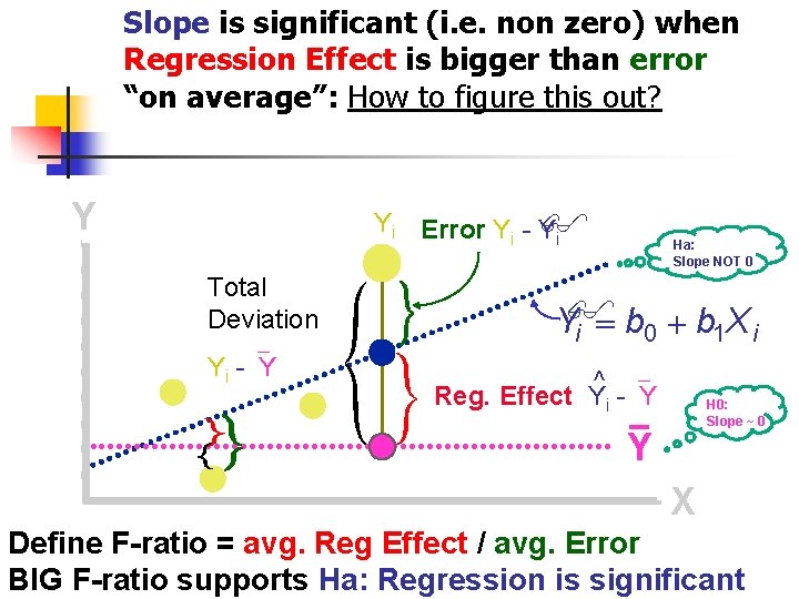
Slope is significant (i. e. non zero) when Regression Effect is bigger than error “on average”: How to figure this out? Y Yi Error Yi - Y i Total Deviation Yi - Y Ha: Slope NOT 0 Yi b 0 b 1 X i ^ Reg. Effect Yi - Y H 0: Slope ~ 0 Y X Define F-ratio = avg. Reg Effect / avg. Error BIG F-ratio supports Ha: Regression is significant

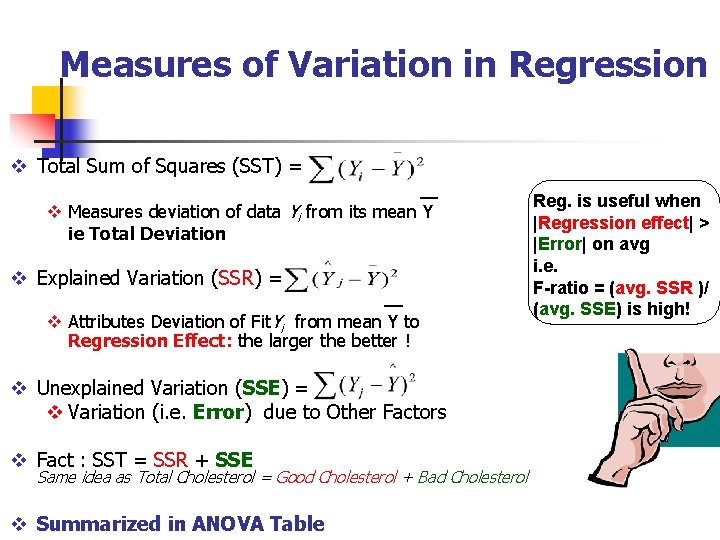
Measures of Variation in Regression v Total Sum of Squares (SST) = v Measures deviation of data Yi from its mean Y ie Total Deviation v Explained Variation (SSR) = v Attributes Deviation of Fit. Yi from mean Y to Regression Effect: the larger the better ! v Unexplained Variation (SSE) = v Variation (i. e. Error) due to Other Factors v Fact : SST = SSR + SSE Same idea as Total Cholesterol = Good Cholesterol + Bad Cholesterol v Summarized in ANOVA Table Reg. is useful when |Regression effect| > |Error| on avg i. e. F-ratio = (avg. SSR )/ (avg. SSE) is high!

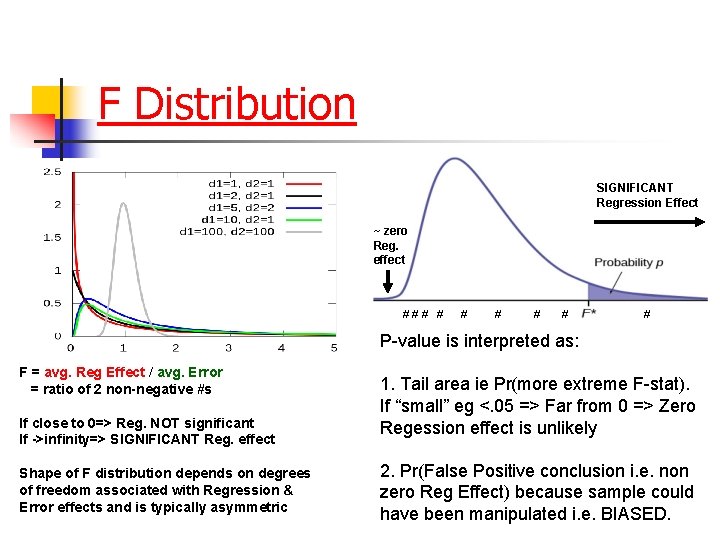
F Distribution SIGNIFICANT Regression Effect ~ zero Reg. effect ### # # # P-value is interpreted as: F = avg. Reg Effect / avg. Error = ratio of 2 non-negative #s If close to 0=> Reg. NOT significant If ->infinity=> SIGNIFICANT Reg. effect Shape of F distribution depends on degrees of freedom associated with Regression & Error effects and is typically asymmetric 1. Tail area ie Pr(more extreme F-stat). If “small” eg <. 05 => Far from 0 => Zero Regession effect is unlikely 2. Pr(False Positive conclusion i. e. non zero Reg Effect) because sample could have been manipulated i. e. BIASED.

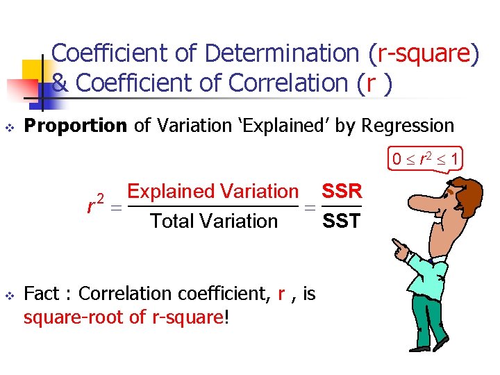
Coefficient of Determination (r-square) & Coefficient of Correlation (r ) v Proportion of Variation ‘Explained’ by Regression 0 r 2 1 2 r v Explained Variation Total Variation Fact : Correlation coefficient, r , is square-root of r-square! SSR SST

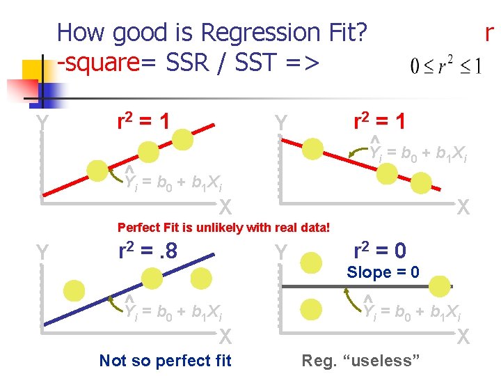
How good is Regression Fit? -square= SSR / SST => Y r 2 = 1 r r 2 = 1 Y ^=b +b X Y i 0 1 i X X Perfect Fit is unlikely with real data! Y r 2 =. 8 Y ^=b +b X Y i 0 1 i r 2 = 0 Slope = 0 ^=b +b X Y i 0 1 i X Not so perfect fit X Reg. “useless”

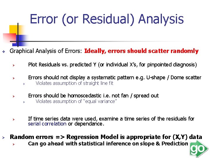
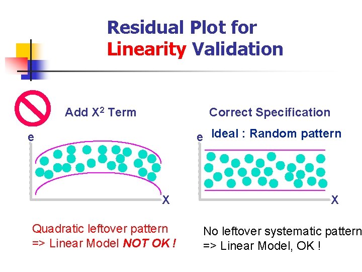
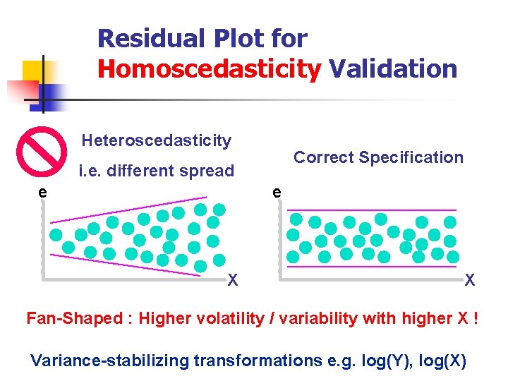
Error (or Residual) Analysis v Graphical Analysis of Errors: Ideally, errors should scatter randomly Ø Plot Residuals vs. predicted Y (or individual X’s, for pinpointed diagnosis) Ø Errors should not display a systematic pattern e. g. U-shape / Dome scatter Ø Errors should be homoscedastic i. e. not fan / spread out Ø Ø Violates assumption of straight line fit Violates assumption of “equal variance” If time series data were used, examine a time series of the residuals for serial correlation or dependance. Random errors => Regression Model is appropriate for (X, Y) data Ø Can go ahead with statistical inference on slope & Prediction

Residual Plot for Linearity Validation Add X 2 Term Correct Specification e Ideal : Random pattern e X Quadratic leftover pattern => Linear Model NOT OK ! X No leftover systematic pattern => Linear Model, OK !

Residual Plot for Homoscedasticity Validation Heteroscedasticity Correct Specification i. e. different spread e e X X Fan-Shaped : Higher volatility / variability with higher X ! Variance-stabilizing transformations e. g. log(Y), log(X)

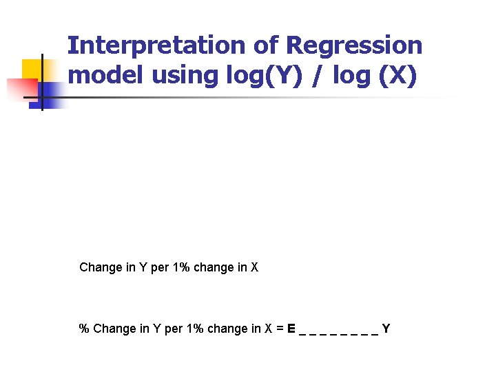
Interpretation of Regression model using log(Y) / log (X) Change in Y per 1% change in X % Change in Y per 1% change in X = E _ _ _ _ Y

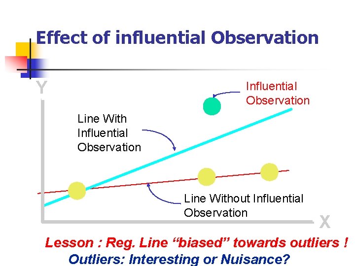
Effect of influential Observation Y Influential Observation Line Without Influential Observation X Lesson : Reg. Line “biased” towards outliers ! Outliers: Interesting or Nuisance?

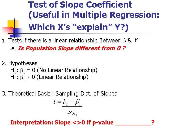
Test of Slope Coefficient (Useful in Multiple Regression: Which X’s “explain” Y? ) 1. Tests if there is a linear relationship Between X & Y i. e. Is Population Slope different from 0 ? 2. Hypotheses H 0: 1 = 0 (No Linear Relationship) H 1: 1 0 (Linear Relationship) 3. Theoretical Basis : Sampling Dist. of Slopes Interpretation: Slope <>0 if p-value _____?

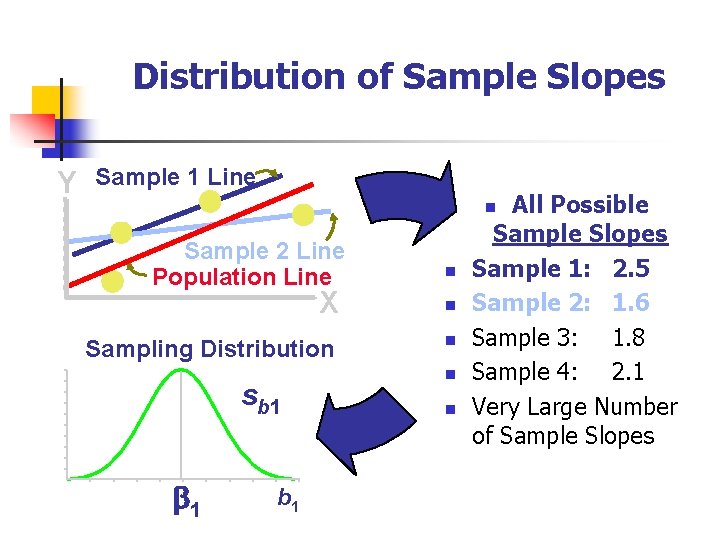
Distribution of Sample Slopes Y Sample 1 Line All Possible Sample Slopes Sample 1: 2. 5 Sample 2: 1. 6 Sample 3: 1. 8 Sample 4: 2. 1 Very Large Number of Sample Slopes n Sample 2 Line Population Line X Sampling Distribution sb 1 1 b 1 n n n

Regression Cautions 1. Violated Assumptions 2. Relevancy of Historical Data 3. Level of Significance 4. Extrapolation 5. Cause & Effect

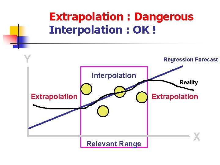
Extrapolation : Dangerous Interpolation : OK ! Y Regression Forecast Interpolation Extrapolation Reality Extrapolation Relevant Range X

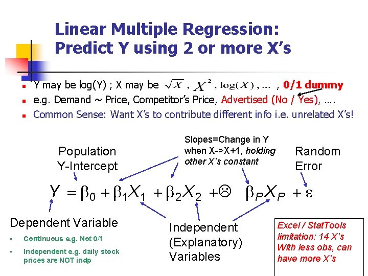
Linear Multiple Regression: Predict Y using 2 or more X’s n n n Y may be log(Y) ; X may be , 0/1 dummy e. g. Demand ~ Price, Competitor’s Price, Advertised (No / Yes), …. Common Sense: Want X’s to contribute different info i. e. unrelated X’s! Population Y-Intercept Slopes=Change in Y when X->X+1, holding other X’s constant Random Error Yi 0 1 X 1 i 2 X 2 i L P X P e i Dependent Variable • Continuous e. g. Not 0/1 • Independent e. g. daily stock prices are NOT indp Independent (Explanatory) Variables Excel / Stat. Tools limitation: 14 X’s With less obs, can have more X’s

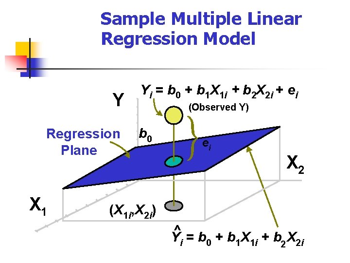
Sample Multiple Linear Regression Model Y Regression Plane X 1 Yi = b 0 + b 1 X 1 i + b 2 X 2 i + ei (Observed Y) b 0 ei X 2 (X 1 i, X 2 i) ^ Yi = b 0 + b 1 X 1 i + b 2 X 2 i

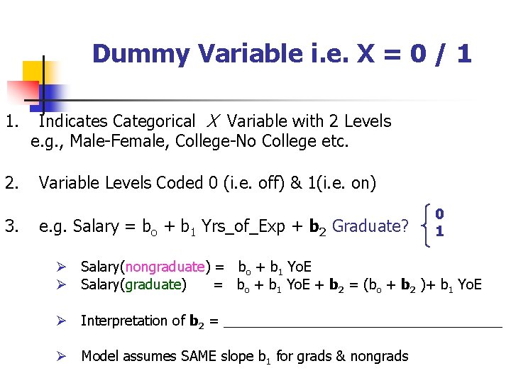
Dummy Variable i. e. X = 0 / 1 1. Indicates Categorical X Variable with 2 Levels e. g. , Male-Female, College-No College etc. 2. Variable Levels Coded 0 (i. e. off) & 1(i. e. on) 3. e. g. Salary = bo + b 1 Yrs_of_Exp + b 2 Graduate? 0 1 Ø Salary(nongraduate) = bo + b 1 Yo. E Ø Salary(graduate) = bo + b 1 Yo. E + b 2 = (bo + b 2 )+ b 1 Yo. E Ø Interpretation of b 2 = __________________ Ø Model assumes SAME slope b 1 for grads & nongrads

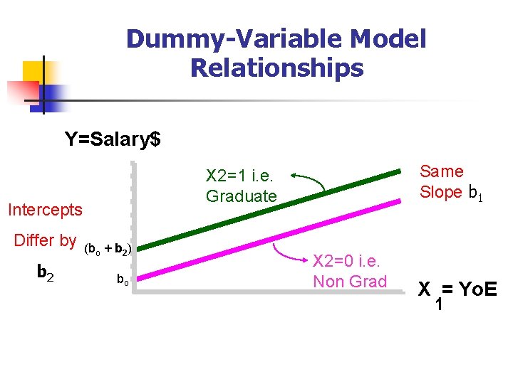
Dummy-Variable Model Relationships Y=Salary$ Intercepts Differ by b 2 Same Slope b 1 X 2=1 i. e. Graduate (bo + b 2) bo X 2=0 i. e. Non Grad X = Yo. E 1

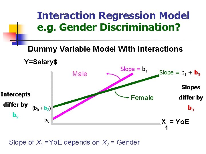
Interaction Regression Model e. g. Gender Discrimination? Dummy Variable Model With Interactions Y=Salary$ Male Slope = b 1 + b 3 Slopes Intercepts differ by b 2 differ by Female b 3 (b 0 + b 2) b 0 X = Yo. E 1 Slope of X 1 =Yo. E depends on X 2 = Gender

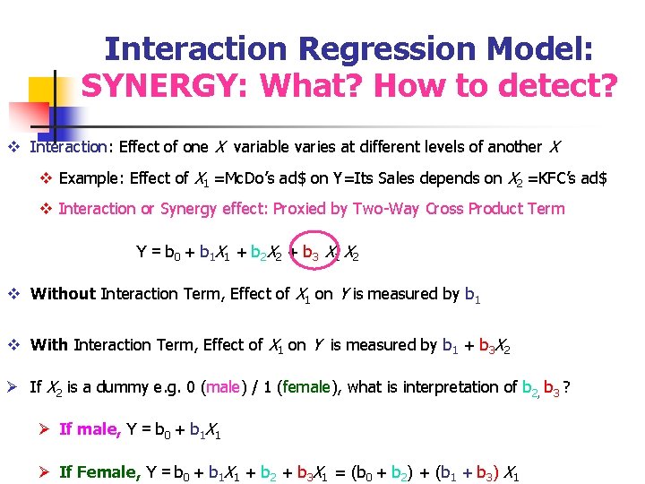
Interaction Regression Model: SYNERGY: What? How to detect? v Interaction: Effect of one X variable varies at different levels of another X v Example: Effect of X 1 =Mc. Do’s ad$ on Y=Its Sales depends on X 2 =KFC’s ad$ v Interaction or Synergy effect: Proxied by Two-Way Cross Product Term Y = b 0 + b 1 X 1 + b 2 X 2 + b 3 X 1 X 2 v Without Interaction Term, Effect of X 1 on Y is measured by b 1 v With Interaction Term, Effect of X 1 on Y is measured by b 1 + b 3 X 2 Ø If X 2 is a dummy e. g. 0 (male) / 1 (female), what is interpretation of b 2, b 3 ? Ø If male, Y = b 0 + b 1 X 1 Ø If Female, Y = b 0 + b 1 X 1 + b 2 + b 3 X 1 = (b 0 + b 2) + (b 1 + b 3) X 1

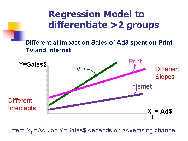
Regression Model to differentiate >2 groups Differential impact on Sales of Ad$ spent on Print, TV and Internet Y=Sales$ Print TV Different Slopes Internet Different Intercepts X = Ad$ 1 Effect X 1 =Ad$ on Y=Sales$ depends on advertising channel

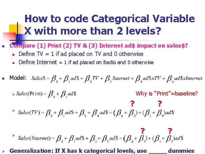
How to code Categorical Variable X with more than 2 levels? n n Compare (1) Print (2) TV & (3) Internet ad$ impact on sales$? n Define TV = 1 if ad placed on TV and 0 otherwise n Define Internet = 1 if ad placed on Radio and 0 otherwise Model: Why is “Print”=baseline? Ø ? ? Ø Ø Ø ? ? Generalization: If X has k categorical levels, use _____ dummies

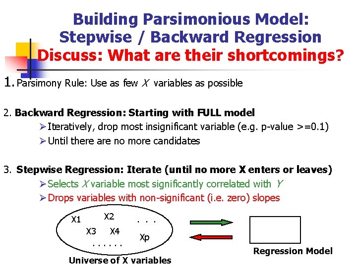
Building Parsimonious Model: Stepwise / Backward Regression Discuss: What are their shortcomings? 1. Parsimony Rule: Use as few X variables as possible 2. Backward Regression: Starting with FULL model Ø Iteratively, drop most insignificant variable (e. g. p-value >=0. 1) Ø Until there are no more candidates 3. Stepwise Regression: Iterate (until no more X enters or leaves) Ø Selects X variable most significantly correlated with Y Ø Drops variables with non-significant (i. e. zero) slopes X 1 X 2 X 3 X 4. . Xp Universe of X variables Regression Model