Refining Core String Edits and Alignments How to

Refining Core String Edits and Alignments

How to find the optimal alignment in linear space

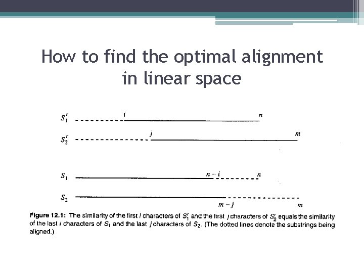
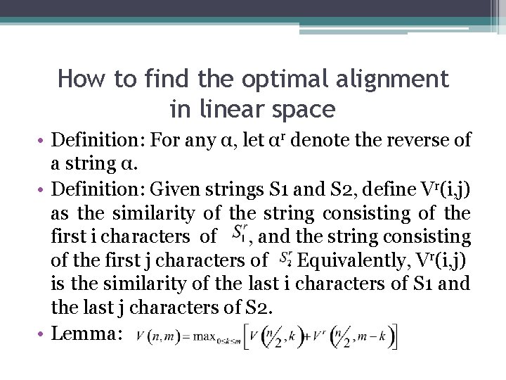
How to find the optimal alignment in linear space • Definition: For any α, let αr denote the reverse of a string α. • Definition: Given strings S 1 and S 2, define Vr(i, j) as the similarity of the string consisting of the first i characters of , and the string consisting of the first j characters of. Equivalently, Vr(i, j) is the similarity of the last i characters of S 1 and the last j characters of S 2. • Lemma:

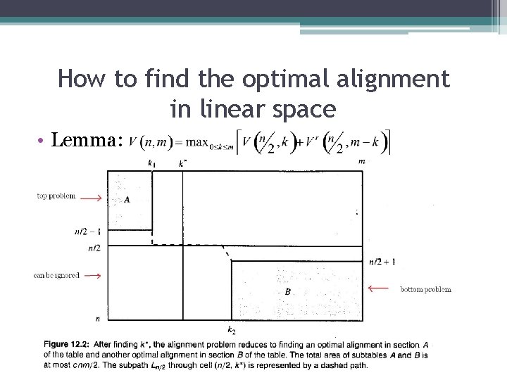
How to find the optimal alignment in linear space • Lemma:

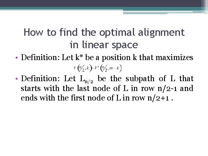
How to find the optimal alignment in linear space • Definition: Let k* be a position k that maximizes • Definition: Let Ln/2 be the subpath of L that starts with the last node of L in row n/2 -1 and ends with the first node of L in row n/2+1.

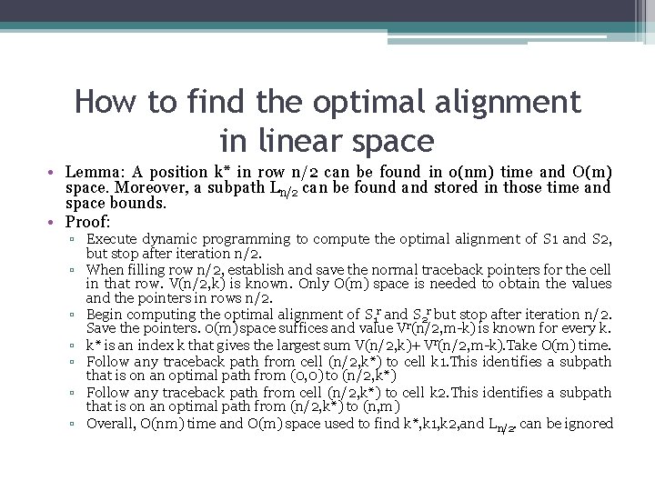
How to find the optimal alignment in linear space • Lemma: A position k* in row n/2 can be found in o(nm) time and O(m) space. Moreover, a subpath Ln/2 can be found and stored in those time and space bounds. • Proof: ▫ Execute dynamic programming to compute the optimal alignment of S 1 and S 2, but stop after iteration n/2. ▫ When filling row n/2, establish and save the normal traceback pointers for the cell in that row. V(n/2, k) is known. Only O(m) space is needed to obtain the values and the pointers in rows n/2. ▫ Begin computing the optimal alignment of S 1 r and S 2 r but stop after iteration n/2. Save the pointers. 0(m) space suffices and value Vr(n/2, m-k) is known for every k. ▫ k* is an index k that gives the largest sum V(n/2, k)+ Vr(n/2, m-k). Take O(m) time. ▫ Follow any traceback path from cell (n/2, k*) to cell k 1. This identifies a subpath that is on an optimal path from (0, 0) to (n/2, k*) ▫ Follow any traceback path from cell (n/2, k*) to cell k 2. This identifies a subpath that is on an optimal path from (n/2, k*) to (n, m) ▫ Overall, O(nm) time and O(m) space used to find k*, k 1, k 2, and Ln/2. can be ignored

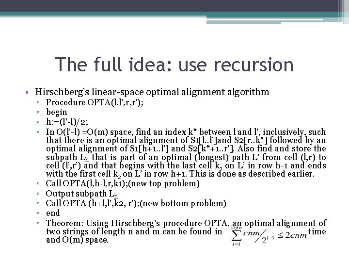
The full idea: use recursion • Hirschberg’s linear-space optimal alignment algorithm ▫ ▫ ▫ ▫ ▫ Procedure OPTA(l, l’, r, r’); begin h: =(l’-l)/2; In O(l’-l) =O(m) space, find an index k* between l and l’, inclusively, such that there is an optimal alignment of S 1[l. . l’]and S 2[r. . k*] followed by an optimal alignment of S 1[h+1. . l’] and S 2[k*+1. . r’]. Also find and store the subpath Lh that is part of an optimal (longest) path L’ from cell (l, r) to cell (l’, r’) and that begins with the last cell k 1 on L’ in row h-1 and ends with the first cell k 2 on L’ in row h+1. This is done as described earlier. Call OPTA(l, h-l, r, k 1); (new top problem) Output subpath Lh Call OPTA (h+l, l’, k 2, r’); (new bottom problem) end Theorem: Using Hirschberg’s procedure OPTA, an optimal alignment of two strings of length n and m can be found in time and O(m) space.

Two specific bounded difference problems • Definition: Given strings S 1 and S 2 and a fixed number k, the k-difference global alignment problem is to find the best global alignment of S 1 and S 2 containing at most k mismatches and spaces (if one exists). • Definition: Given strings P and T, the k-difference inexact matching problem is to find all ways (if any) to match P in T using at most k character substitutions, insertions, and deletions. That is, find all occurrences of P in T using at most k mismatches and spaces. (End spaces in T but not P are free).

k-difference global alignment

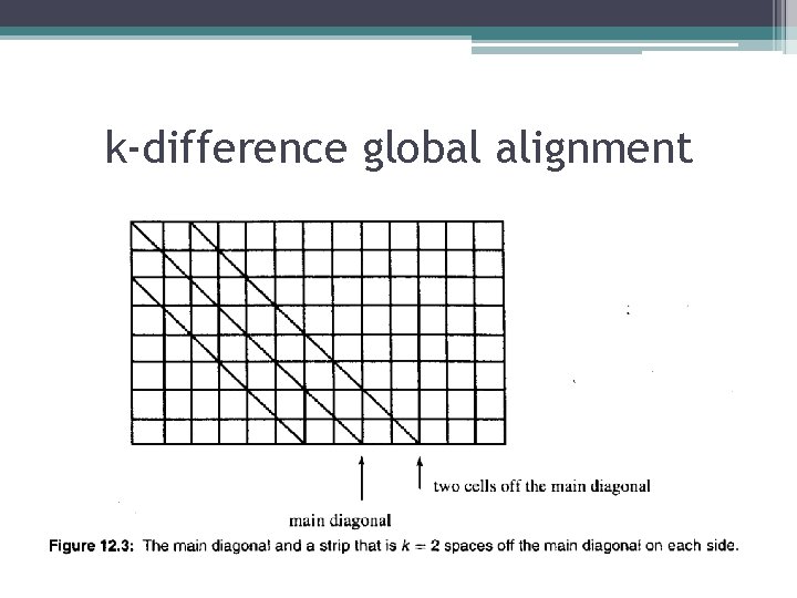
k-difference global alignment • Define the main diagonal of the dynamic programming table as the cells (i, i) for i<=n<=m, then any path in the dynamic programming table that defines a kdifference global alignment must not contain any cell (i, i+l) or (i, i-l) where l>k. • Any path specifying a global alignment begins on the (0, 0) and ends on, or to the right of the main diagonal (in cell (n, m))=>the path must introduce one space in the alignment for every horizontal move that the path makes off the main diagonal. • But, only those paths that are never more than k horizontal cells from the main diagonal are candidates for specifying a k-difference global alignment. =>m-n<=k is a necessary condition for there to be any solution. • To find any k-difference global alignment, it suffices to fill the dynamic programming table in a strip consisting of 2 k+1 cells ub each row, centered on the main diagonal. • When assigning values to cells in that strip, the algorithm follows the established recurrence relations fir edit distance except for cells in the upper and lower border of the strip. Any cell on the upper border of the strip ignores the term in the recurrence relation for the cell above(since it is out of the strip); similarly, any cell on the lower border ignores the term in the recurrence relation for the cell to the left.

k-difference global alignment • Theorem: There is a global alignment of S 1 and S 2 with at most k differences if and only if the above algorithm assigns a value of k or less to cell(n, m). Hence the k-difference global alignment problem can be solved in O(km) time and O(km) space.

What if k is not specified? • Theorem: By successively doubling k until there is a k-difference global alignment, the edit distance k* and its associated alignment are computed in O(k*m) time and space. • Proof: Let k’ be the largest value of k used in the method. Clearly, k’ <=2 k*(because the alignment paths are divided into two types: those contained entirely in the present strip and those that go out of the strip). So the total work in the method is O(k’m+k’m/2+k’m/4+…+m) = O(k’m)=O(k*m)

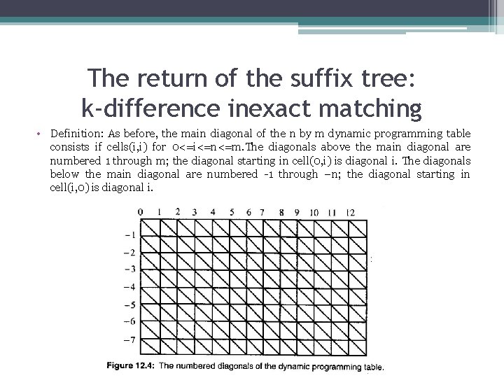
The return of the suffix tree: k-difference inexact matching • Definition: As before, the main diagonal of the n by m dynamic programming table consists if cells(i, i) for 0<=i<=n<=m. The diagonals above the main diagonal are numbered 1 through m; the diagonal starting in cell(0, i) is diagonal i. The diagonals below the main diagonal are numbered -1 through –n; the diagonal starting in cell(i, 0) is diagonal i.

The return of the suffix tree: k-difference inexact matching • Definition: A d-path in the dynamic programming table is a path that starts in row zero and specifies a total of exactly d mismatches and spaces. • Definition: A d-path is farthest-reaching in diagonal i if it is a d-path that ends in diagonal i, and the index of it’s ending column c (along diagonal i) is greater than or equal to the ending column of any other d-path ending in diagonal i.

Hybrid dynamic programming : the high-level idea • In every iteration d<=k, the method finds the end of the farthest-reaching d-path on diagonal i, for each i from –n to m. The farthest-reaching d-path on diagonal i is found from the farthest-reaching (d-1)-paths on diagonals i-1, i, i+1. • Details: ▫ When d=0, the farthest-reaching 0 -path ending on diagonal i corresponds to the longest common extension of T[i. . m] and P[1. . n], since a 0 -path allows no mismatches or spaces. =>can be found in constant time. ▫ For d>0, the farthest-reaching d-path on diagonal I can be found by considering the following three particular paths that end on diagonal i.

Hybrid dynamic programming : the high-level idea

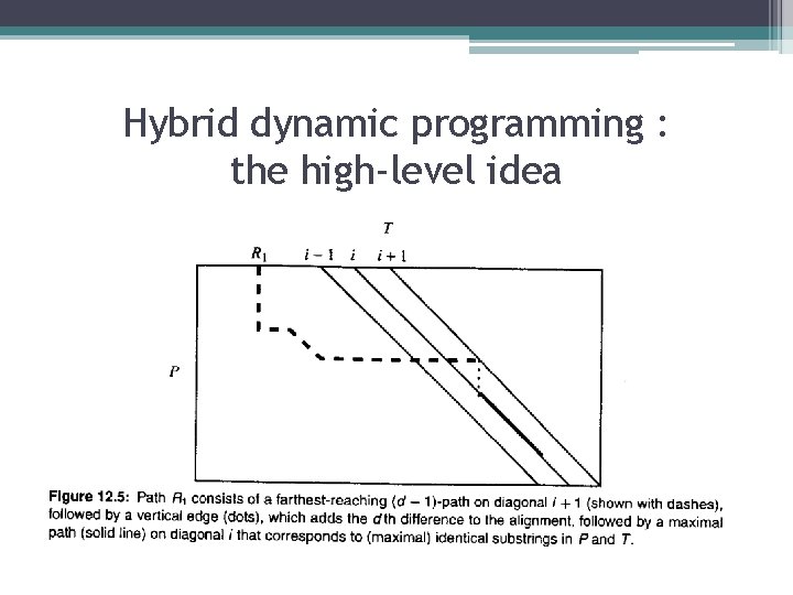
Hybrid dynamic programming : the high-level idea • Path R 1 consists of the farthest-reaching (d-1) –path on diagonal i+1, followed by a vertical edge (a space in text T) to diagonal i, followed by the maximal extension along diagonal i that corresponds to identical substrings in P and T. Since R 1 begins with a (d-1)-path and adds one more space for the vertical edge, R 1 is a d-path. • Path R 1 consists of the farthest-reaching (d-1) –path on diagonal i-1, followed by a horizontal edge (a space in pattern P) to diagonal i, followed by the maximal extension along diagonal i that corresponds to identical substrings in P and T. Path R 2 is a d-path. • Path R 3 consists of the farthest-reaching (d-1) –path on diagonal i, followed by a diagonal edge corresponding to a mismatch between a character of P and a character of T, followed by the maximal extension along diagonal i that corresponds to identical substrings in P and T. Path R 3 is a d-path.

Hybrid dynamic programming : the high-level idea

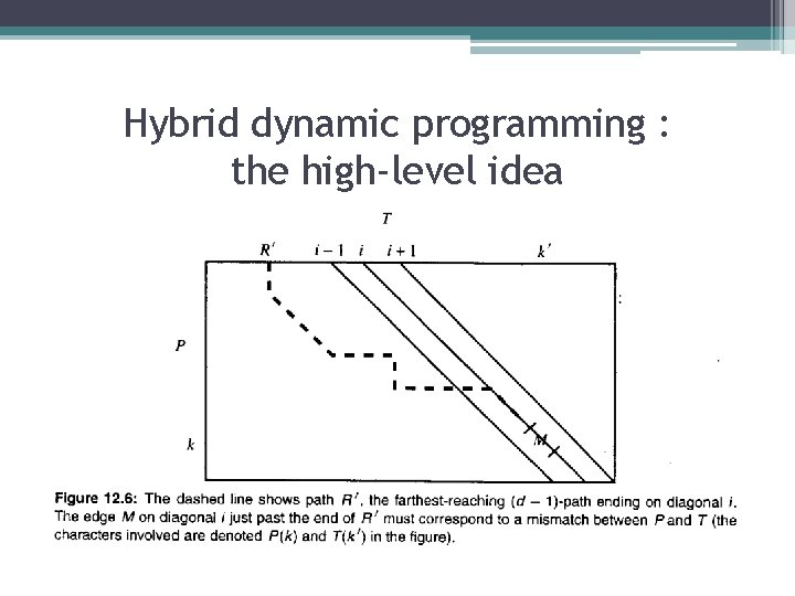
Hybrid dynamic programming : the high-level idea • In the case of R 1(or R 2), the starting positions of the two substrings are given by the last entry point of R 1(or R 2) into diagonal i. In the case of R 3, the starting position is the position just past the last mismatch on R 3. • Theorem: Each of the three paths R 1, R 2 and R 3 are d-paths ending on diagonal i. The farthestreaching d-path on diagonal i is the path R 1, R 2, or R 3 that extends the farthest along diagonal i.

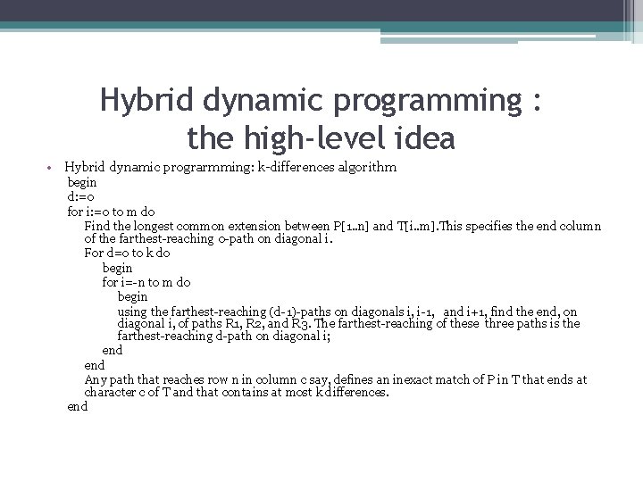
Hybrid dynamic programming : the high-level idea • Hybrid dynamic prograrmming: k-differences algorithm begin d: =0 for i: =0 to m do Find the longest common extension between P[1. . n] and T[i. . m]. This specifies the end column of the farthest-reaching 0 -path on diagonal i. For d=o to k do begin for i=-n to m do begin using the farthest-reaching (d-1)-paths on diagonals i, i-1, and i+1, find the end, on diagonal i, of paths R 1, R 2, and R 3. The farthest-reaching of these three paths is the farthest-reaching d-path on diagonal i; end Any path that reaches row n in column c say, defines an inexact match of P in T that ends at character c of T and that contains at most k differences. end

Implementation and time analysis • Theorem: All locations in T where pattern P occurs with at most k differences can be found in O(km)-time and O(km) space. Moreover, the actual alignment of P and T for each of these locations can be reconstructed in O(km) total time. • Theorem: In O(km)-time and O(n+m) space, the algorithm can find all the end locations in T where P matches T with at most k differences

The primer (and probe) selection problem revisited – An application of bounded difference matching • Exact matching primer (and probe) problem : For each index j past some starting point, find the shortest substring γ of α (if any) that begins at position j and that does not appear as a substring of β. • Definition: Primers are short substrings of DNA that hybridize to the desired part of string α and that ideally should not hybridize to any parts of another string β. • Inexact matching primer problem: Given a parameter p, find for each index j (past some starting point), the shortest substring γ of α (if any) that begins at position j and that has edit distance at least |γ|/p from any substring in β. • k-difference primer problem: Given a parameter p, find for each index j (past some starting point), the shortest substring γ of α (if any) that begins at position j and that has edit distance at least k from any substring in β. • Changing |γ|/p to k in the problem statement makes the solution easier but does not reduce the utility of the solution. The reason is that the length of a practical primer must be within a fixed and fairly narrow range, so for fixed p, |γ|/p also falls in a small range. Hence for a specified p, the k-difference primer problem can be solved for a small range of choices for k and still be expected to pick out useful primer candidates.

How to solve the k-difference primer problem • For any position j, the k-difference primer problem becomes: ▫ Find the shortest prefix of string α[j. . n] (if it exists) that has edit distance at least k from every substring in β. • Solution: ▫ Run the k-differences algorithm with string α[j. . n] playing the role of P and β playing the role of T. • Theorem: If α has length n and β has length m, then the k-differences primer selection problem can be solved in O(knm) total time.

Exclusion methods: fast expected running time • Partition approach to approximate matching ▫ Partition T or P into consecutive regions of a given length r (to be specified later). ▫ Search phase Using various exact matching methods, search T to find length-r intervals of T (or regions, if T was partitioned) that could be contained in an approximate occurrence of P. These are called surviving intervals. The nonsurviving intervals are definitely not contained in any approximate occurrence of P, and the goal of this phase is to eliminate as many intervals as possible. ▫ Check phase For each surviving interval R of T, use some approximate matching method to explicitly check if there is an approximate occurrence of P in a larger interval around R. • The point of the partition approach is to exclude a large amount of T, using only (sub)linear expected time in the search phase, so that only (sub)linear expected time is needed to check the few surviving intervals. A balance is needed between searching and checking because a reduction in the time used in one phase causes an increase in the time used in the other phase.

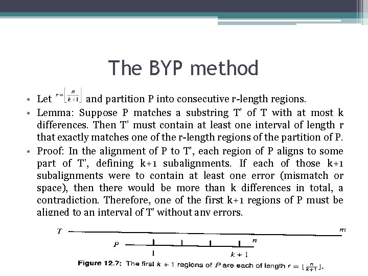
The BYP method • Let and partition P into consecutive r-length regions. • Lemma: Suppose P matches a substring T’ of T with at most k differences. Then T’ must contain at least one interval of length r that exactly matches one of the r-length regions of the partition of P. • Proof: In the alignment of P to T’, each region of P aligns to some part of T’, defining k+1 subalignments. If each of those k+1 subalignments were to contain at least one error (mismatch or space), then there would be more than k differences in total, a contradiction. Therefore, one of the first k+1 regions of P must be aligned to an interval of T’ without any errors.

The BYP method • Algorithm BYP ▫ Let P be the set of k+1 substrings of P taken from the first k+1 regions of P’s partition. ▫ Build a keyword tree for the set of “patterns” P. ▫ Using the Aho-Corasik algorithm, find I, the set of all starting locations in T where any pattern in P occurs exactly. ▫ For each index use an approximate matching algorithm (usually based on dynamic programming) to locate the end points of all approximate occurrences of P in the substring T[i-n-k. . i+n+k] (i. e. , in an appropriate-length interval around i)

Expected time analysis of algorithm BYP • Steps b, c run in O(m) • Each character of T is drawn uniformly from an alphabet of size σ. P can be an arbitrary string. Consider any pattern p. EP. p has length r and T contains roughly m substrings of length r, the expected number of exact occurrences of p in T is m/σr. =>The expected total number of occurrences in T of patterns from P is m(k+1)/σr. • For each i. EI, the algorithm spends O(n 2) time in checking phase=>The expected checking time is mn 2 (k+1)/σr. =>We want be linear=> mn 2 (k+1)/σr <cm. Replace k by n-1=> mn 3 /σr =cm. =>σr=n 3/c, r=logσn 3 logσc. But • Algorithm BYP runs in O(m) time for k=O(n/logn)

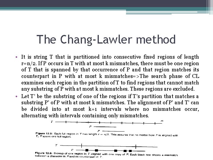
The Chang-Lawler method • It is string T that is partitioned into consecutive fixed regions of length r=n/2. If P occurs in T with at most k mismatches, there must be one region of T that is spanned by that occurrence of P and that region matches its counterpart in P with at most k mismatches=>The search phase of CL examines each region in the partition of T to find regions that cannot match any substring of P with at most k mismatches. These regions are excluded. • Let T’ be the substring of one of the regions if T’s partition that matches a substring P’ of P with at most k mismatches. The alignment of P’ and T’ can be divided into at most k+1 intervals where no mismatches occur, alternating with intervals containing only mismatches.

The Chang-Lawler method • The CL search in region R ▫ ▫ ▫ ▫ Set j to the starting position j* of region R in T cn: =0; Repeat Compute ms(j); J: =j+ms(j)+1; cn: =cn+1; Until cn=k or j-j* >n/2 If j-j* > n/2 then region R survives, otherwise it is excluded • If R is a surviving region, then in the checking phase CL executes an approximate matching algorithm for P against a neighborhood of T that starts n/2 positions to the left of R and ends n/2 positions to its right. • Lemma: When the CL search declares a region R excluded, then there is no occurrence of P in T with at most k mismatches that completely contains region R

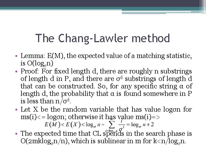
The Chang-Lawler method • Lemma: E(M), the expected value of a matching statistic, is O(logσn) • Proof: For fixed length d, there are roughly n substrings of length d in P, and there are σd substrings of length d that can be constructed. So, for any specific string α of length d, the probability that α is found somewhere in P is less than n/σd. • Let X be the random variable that has value logσn for ms(i)<= logσn; otherwise it has value ms(i)=> • The expected time that CL spends in the search phase is O(2 mklogσn/n), which is sublinear in m for k<n/logσn.

Multiple filtration for k-mismatches • Myers’s sublinear-time method ▫ Contains two different ideas to make it both selective (finding fewer initial surviving regions) and less expensive to test the ones that are found. ▫ It partitions P into short substrings and then finds all locations in T where these substrings appear with a smaller number of allowed differences. ▫ The detail of the search are quite different from the other methods, but the intent (to exclude a large portion of T from further consideration) is the same. Each of these initial alignments of a substring of P that is found in T is called a surviving match. ▫ After it will incrementally extend and check a growing interval around each initial surviving match to create a longer surviving matches or to exclude a surviving match from further consideration. This is done in about O(logn) iterations.

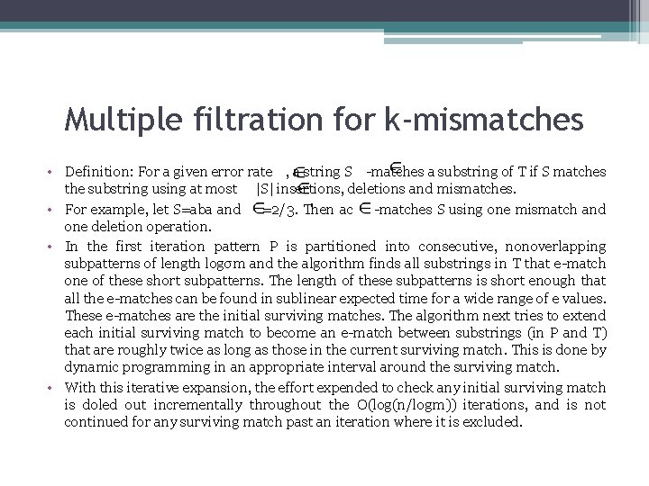
Multiple filtration for k-mismatches • Definition: For a given error rate , a string S -matches a substring of T if S matches the substring using at most |S| insertions, deletions and mismatches. • For example, let S=aba and =2/3. Then ac -matches S using one mismatch and one deletion operation. • In the first iteration pattern P is partitioned into consecutive, nonoverlapping subpatterns of length logσm and the algorithm finds all substrings in T that e-match one of these short subpatterns. The length of these subpatterns is short enough that all the e-matches can be found in sublinear expected time for a wide range of e values. These e-matches are the initial surviving matches. The algorithm next tries to extend each initial surviving match to become an e-match between substrings (in P and T) that are roughly twice as long as those in the current surviving match. This is done by dynamic programming in an appropriate interval around the surviving match. • With this iterative expansion, the effort expended to check any initial surviving match is doled out incrementally throughout the O(log(n/logm)) iterations, and is not continued for any surviving match past an iteration where it is excluded.

The first iteration • Definition: For a string S and value of e , let d = e|Sl. The d-neighborhood of S is the set of all strings that e-match S. • For example, over the twο-letter alphabet {a, b}, it S =αbα and d=1, then the 1 -neighborhood of S is {bbα, ααα, αbb, ααbα, αbαα, bαbα, αbαb, bα, αb}. Ιt is created from S by the operations of mismatch, insertion and deletion respectively. The condensed d-neighborhood of S is created from the d-neighborhood of s by removing any substring that is a prefix of another string in the d-neighborhood. The condensed 1 -neighborhoοd S is {bbα, ααbα, αbαα, bαbα, αbαb}. • Recall that pattern P is initially partitioned into subpatterns of length logσm (assumed to be an integer). Let P be the set of these subpatterns. In the first iteration, the algorithm (conceptuaΙly) constructs the condensed d-neighborhood for each subpattern in P, and then finds all locations of substrings in text T that exactly match one of the substrings in one of the condensed dneighborhoods. In this way, the method T finds all substrings of T that e-match one of the subpatterns in P. These ε-matches form the initial surviving matches. • In actuality, the tasks of generating the substrings in the condensed d-neighborhoods and of searching for their exact occurrences in T are intertwined and require text T to have been preprocessed into some index structure. This structure could be a suffix tree, a suffix array or a hash table holding short substrings of T. • Myers shows that when the length of the subpatterns is o(logσm), then the first iteration can be implemented to run in o(kmp(e)logm) expected time. The function p(e) is complicated, but it is convex (negative second derivative) increasing, and increases more slowly as the alphabet size grows.

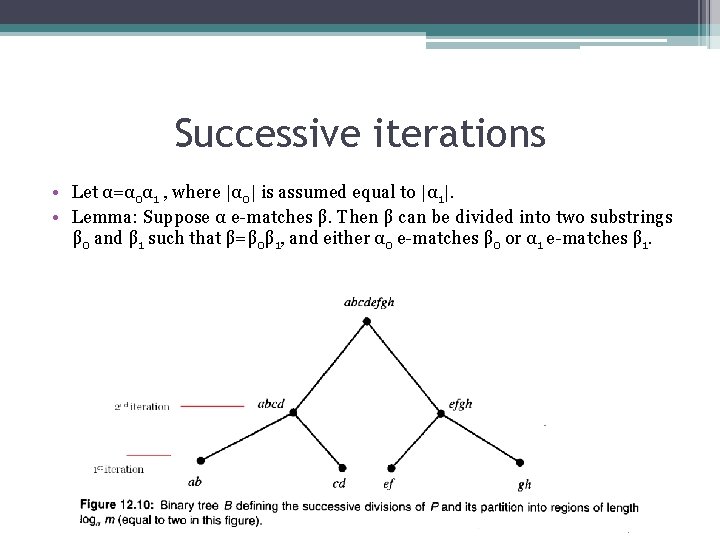
Successive iterations • Let α=α 0α 1 , where |α 0| is assumed equal to |α 1|. • Lemma: Suppose α e-matches β. Then β can be divided into two substrings β 0 and β 1 such that β=β 0β 1, and either α 0 e-matches β 0 or α 1 e-matches β 1.

Final comments on Myers’s method • Unlike the BYP and CL methods, the error rates that establish sublinear running times do not depend on the length of P. The permitted error rate depends only on the alphabet size. • In CL method, the sublinearity is due to a multiplicative factor that is less than one. In Myers’s method, the sublinearity is due to a exponent that is less than one. =>so as a function of m, the CL bound increases linearly, while the bound for the Myers’s method increases sublinearly in m. • Assumes that the text T has already been preprocessed into some index structure.

Yet more suffix trees and more hybrid dynamic programming • Two problems ▫ The P-against-all problem Given strings P and T, compute the edit distance between P and every substring T’ of T. ▫ The threshold all-against-all problem Given strings P and T and a threshold d, find every pair of substrings P’ of P and T’ of T such that the edit distance between P’ and T’ is less than d.

The P-against-all problem • The P-against-all problem is an example of a large-scale alignment problem that asks for a great amount of related alignment information. • Let P has length n and T has length m>n. Naïve solution: enumerate all substrings of T, and then separately compute the edit distance between P and each substring of T. =>Θ(nm 3) • We need only choose each suffix S of T and compute the dynamic programming edit distance table for strings P and S. If S begins at position i of T , then the last row of that table gives the edit distance between P and every substring of T that begins at position i. That is, the edit distance between P and T[i. . i] is found in cell(n, j - i + 1) of the table. =>Θ(nm 2)

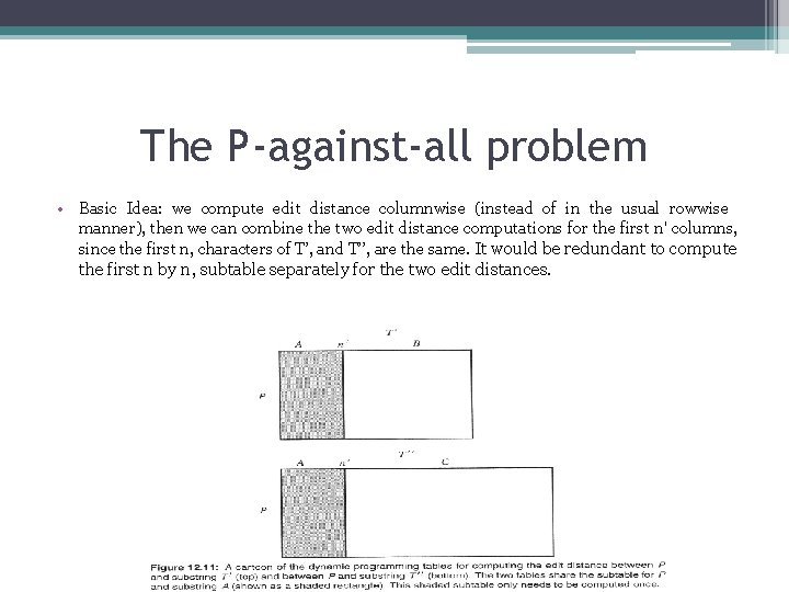
The P-against-all problem • Basic Idea: we compute edit distance columnwise (instead of in the usual rowwise manner), then we can combine the two edit distance computations for the first n' columns, since the first n, characters of T’, and T’’, are the same. It would be redundant to compute the first n by n, subtable separately for the two edit distances.

The P-against-all problem

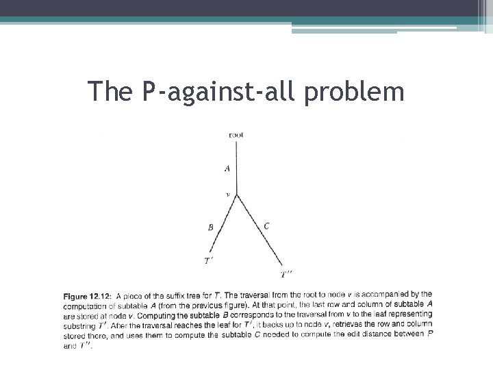
The P-against-all problem • Definition: The string-length of an edge label in a suffix tree is the length of the string labeling that edge (even though the label is compactly represented by a constant number of characters). The length of a suffix tree is the sum of the string-lengths for all of its edges. • Lemma: The time used to generate the needed columns in the depth-first traversal is Θ[n(length of T)]. • Theorem: The totαl time for the suffix-tree approach is Θ(n x(length of T)+m 2) and the maximum space used is Θ(m. ). • Theorem: The hybrid suffix-tree /dynamic programming approach to the P-against-all problem can be implemented to run in Θ[n(length of T) + m 2] time and O(n+m) space.

The (threshold) all-against-all problem • Given strings P and T, find every pair of substrings where the edit distance is below a fixed threshold d. No method for this problem can run faster than Θ(n 2 m 2) time. • Pick a pair of Starting positions in Ρ and T (in nm possible ways), and for each choice of starting positions i, j fill in the dynamic programming table for the edit distance of P[i. . n] and T [j. . m] (in O(nm)-time). For any choice of j and j , the entries in the corresponding tab 1 e give the edit distance for every pair of substrings that begin at position j in P and at position j in T. • Calls for an amount of output that is often excessive, and the output can be reduced by choosing a meaningful threshold. =>we develop a method whose worst-case running time is expressed as O(C + R), where C is a computation time that may be less than Θ(n 2 m 2) and R is the output size (i. e. , the number of reported pairs of substrings).

An O(C + R)-time methοd • The method uses a suffix tree Tp for string P and a suffix tree TT for string T. The worst-case time for the method will be shown to be O(C+R), where C is the length of Tp times the length of TT independent of whatever the output criteria are, and R is the size οf the output. • Definition: The dynamic programming table for a pair of nodes (u, v), from Tp and TT, respectively, is defined as the dynamic programming table for the edit distance between the string represented by node u and the string represented by node v.

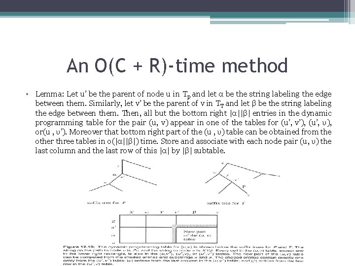
An O(C + R)-time methοd • Lemma: Let u’ be the parent of node u in Tp and let α be the string labeling the edge between them. Similarly, let v’ be the parent of v in TT and let β be the string labeling the edge between them. Then, all but the bottom right |α||β| entries in the dynamic programming table fοr the pair (u, v) appear in one of the tables fοr (u’, v’), (u’, υ), οr(u , υ’). Moreover that bottom right part of the (u , υ) table can be obtained from the other three tables in o(|α||β|) time. Store and associate with each node pair (u, υ) the last column and the last row of this |α| by |β| subtable.

Correctness and time analysis • The correctness of the method follows from the fact that at the highest level of description, the method computes the edit distance for every pair of substrings, one from each string. It does this by generating and examining every cell in the dynamic programming table for every pair of substrings (although it avoids redundant examinations). The only subtle point is that the method generates and examines the cells in each table in an incremental manner to exploit the commonalities between substrings, and hence it avoids regenerating and reexamining any cell that is part of more than one table. Further when the method finds a cell satisfying the reporting criteria (a function of value and length), it can find all the pairs of substrings specified by that cell using a traversal to a subset of leaves in the two suffix trees.

Correctness and time analysis • Lemma: The time used by the algorithm for all the needed dynamic programming computations and cell examinations is proportional to the product of the length of Tp and the length of TT. Hence that time, defined as C, ranges between nm and n 2 m 2. • Proof: In the algorithm, each pair of nodes is processed exactly once. At the point a pair (u, υ) is processed, the algorithm spends O(|α||β|) time to compute a subtable and examine it, where α and β are the labels on the edges into u and v, respectively. Each edge-label in Tp therefore forms exactly one dynamic programming table with each of the edge-labels in TT. The time to build those tables is |α|(length of TT). Summing over all edges in Tp gives the claimed time bound. • Theorem: The complete time for the algorithm is O(C + R).

A faster (combinatorial) algorithm for longest common subsequence • The longest common subsequence problem (lcs) is a special case of general weighted alignment or edit distance, and it can be solved in Θ(nm) time. • We present an alternative (combinatorial) method for lcs that is not based on dynamic programming. The main idea is to reduce the lcs problem to a longest increasing subsequence problem (lis). • Definition: Let Π be a list of n integers, not necessarily distinct. An increasing subsequence of Π is a subsequence of Π whose values strictly increase from left to right. • Definition: A decreasing subsequence of Π is a subsequence of Π where the numbers are nonicreasing from left to right. • Definition: A cover of Π is a set of decreasing subsequences of Π that contain all the numbers of Π. • Definition: The size of the cover is the number of decreasing subsequences in it, and a smallest cover is a cover with minimum size among all covers.

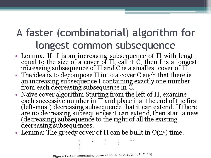
A faster (combinatorial) algorithm for longest common subsequence • Lemma: If I is an increasing subsequence of Π with length equal to the size of a cover of Π, call it C, then I is a longest increasing subsequence of Π and C is a smallest cover of Π. • The idea is to decompose Π in tο a cover C such that there is an increasing subsequence I containing exactly one number from each decreasing subsequence in C. • Naïve cover algorithm Starting from the left of Π, examine each successive number in Π and place it at the end of the first (left-most) decreasing subsequence that it can extend. If there are no decreasing subsequences it can extend, then start a new (decreasing) subsequence to the right of all the existing decreasing subsequences. • Lemma: The greedy cover of Π can be built in O(n 2) time.

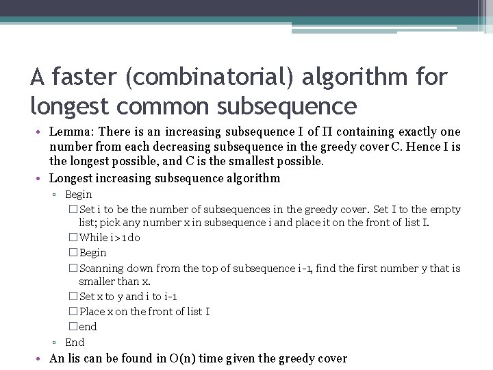
A faster (combinatorial) algorithm for longest common subsequence • Lemma: There is an increasing subsequence I of Π containing exactly one number from each decreasing subsequence in the greedy cover C. Hence I is the longest possible, and C is the smallest possible. • Longest increasing subsequence algorithm ▫ Begin � Set i to be the number of subsequences in the greedy cover. Set I to the empty list; pick any number x in subsequence i and place it on the front of list I. � While i>1 do � Begin � Scanning down from the top of subsequence i-1, find the first number y that is smaller than x. � Set x to y and i to i-1 � Place x on the front of list I � end ▫ End • An lis can be found in O(n) time given the greedy cover

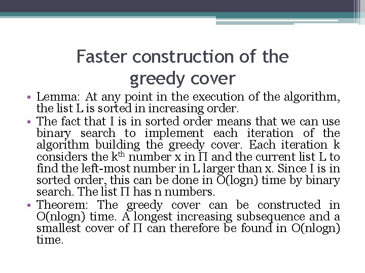
Faster construction of the greedy cover • Lemma: At any point in the execution of the algorithm, the list L is sorted in increasing order. • The fact that Ι is in sorted order means that we can use binary search to implement each iteration of the algorithm building the greedy cover. Each iteration k considers the kth number x in Π and the current list L to find the left-mοst number in L larger than x. Since Ι is in sorted order, this can be done in O(logn) time by binary search. The list Π has n numbers. • Theorem: The greedy cover can be constructed in O(nlogn) time. A longest increasing subsequence and a smallest cover of Π can therefore be found in O(nlogn) time.

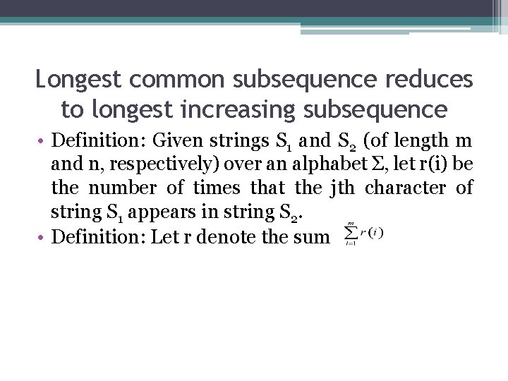
Longest common subsequence reduces to longest increasing subsequence • Definition: Given strings S 1 and S 2 (of length m and n, respectively) over an alphabet Σ, let r(i) be the number of times that the jth character of string S 1 appears in string S 2. • Definition: Let r denote the sum

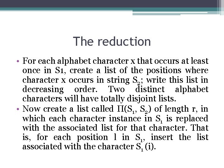
The reduction • For each alphabet character x that occurs at least once in S 1, create a list of the positions where character x occurs in string S 2; write this list in decreasing order. Two distinct alphabet characters will have totally disjoint lists. • Now create a list called Π(S 1, S 2) of length r, in which each character instance in S 1 is replaced with the associated list for that character. That is, for each position l in S 1, insert the list associated with the character S 1 (i).

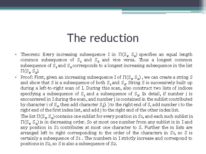
The reduction • Theorem: Every increasing subsequence Ι in Π(S 1, S 2) specifies an equal length common subsequence of S 1 and S 2 and vice versa. Thus a longest common subsequence of S 1 and S 2 corresponds to a longest increasing subsequence in the list Π(S 1, S 2). • Proof: First, given an increasing subsequence I of Π(S 1, S 2) , we can create a string S and show that S is a subsequence of both S 1 and S 2. String S is successively built up during a left-to-right scan of I. During this scan, also construct two lists of indices specifying a subsequence of S 1 and a subsequence of S 2. In detail, if number j is encountered in I during the scan, and number j is contained in the sublist contributed by character i of S 1, then add character S 1(i ) to the right end of S, add number i to the right end of the first index list, and add j to the right end of the other index list. The list Π(S 1, S 2) contains one sublist for every position in S 1, and each sublist in Π(S 1, S 2) is in decreasing order. So at most one number from any sublist is in I and any position in S 1 contributes at most one character to S. Further the m lists are arranged left to right corresponding to the order of the characters in S 1, so S is certainly a subsequence of S 1. The numbers in I strictly increase and correspond to positions in S 2, so S is also a subsequence of S 2.

The reduction • Theorem: The longest Common subsequence problem can be solved in O(rlogn)time.

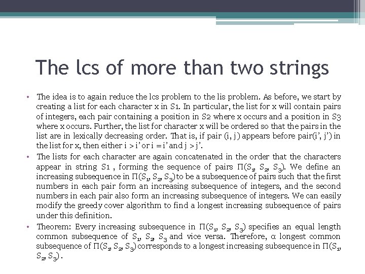
The lcs of more than two strings • The idea is to again reduce the lcs problem to the lis problem. Αs before, we start by creating a list for each character x in S 1. In particular, the list for x will contain pairs of integers, each pair containing a position in S 2 where x occurs and a position in S 3 where x occurs. Further, the list for character x will be ordered so that the pairs in the list are in lexically decreasing order. That is, if pair (i, j) appears before pair(i’, j’) in the list for x, then either i > i’ or i = i’ and j > j’. • The lists for each character are again concatenated in the order that the characters appear in string S 1 , forming the sequence of pairs Π(S 1, S 2, S 3). We define an increasing subsequence in Π(S 1, S 2, S 3) to be a subsequence of pairs such that the first numbers in each pair form an increasing subsequence of integers, and the second numbers in each pair also form an increasing subsequence of integers. We can easily modify the greedy cover algorithm to find a longest increasing subsequence of pairs under this definition. • Theorem: Every increasing subsequence in Π(S 1, S 2, S 3) specifies an equal length common subsequence of S 1, S 2, S 3 and vice versa. Therefore, α longest common subsequence of Π(S 1, S 2, S 3) corresponds to a longest increasing subsequence in Π(S 1, S 2, S 3).

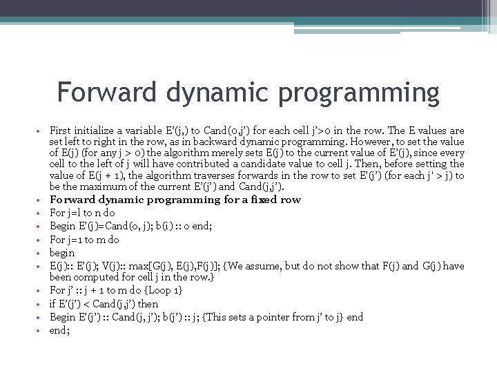
Forward dynamic programming • First initialize a variable Ε’(j, ) to Cand(0, j’) for each cell j’>0 in the row. The E values are set left to right in the row, as in backward dynamic programming. However, to set the value of E(j) (for any j > 0) the algorithm merely sets E(j) to the current value of E’(j), since every cell to the left of j will have contributed a candidate value to cell j. Then, before setting the value of Ε(j + 1), the algorithm traverses forwards in the row to set E’(j’) (for each j' > j) to be the maximum of the current E’(j’) and Cand(j, j’). • Forward dynamic programming for a fixed row • For j=l to n do • Begin Ε’(j)=Cand(o, j); b(i) : : o end; • For j=1 tο m do • begin • Ε(j): : E’(j); V(j): : max[G(j), Ε(j), F(j)]; {We assume, but do not show that F(j) and G(j) have been computed for cell j in the row. } • For j’ : : j + 1 to m do {Lοop 1} • if Ε’(j’) < Cand(j, j’) then • Begin Ε’(j’) : : Cand(j, j’); b(j’) : : j; {This sets a pointer from j’ to j} end • end;

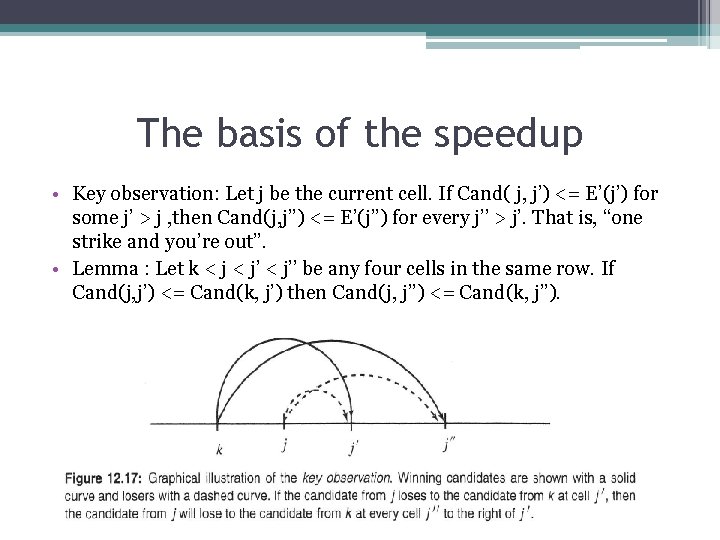
The basis of the speedup • Key observation: Let j be the current cell. Ιf Cand( j, j’) <= Ε’(j’) for some j’ > j , then Cand(j, j’’) <= E’(j’’) for every j’’ > j’. That is, “one strike and you’re out”. • Lemma : Let k < j’’ be any four cells in the same row. Ιf Cand(j, j’) <= Cand(k, j’) then Cand(j, j’’) <= Cand(k, j’’).

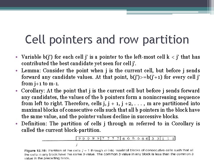
Cell pointers and row partition • Variable b(j') for each cell j’ is a pointer to the left-most cell k < j’ that has contributed the best candidate yet seen for cell j’. • Lemma: Consider the point when j is the current cell, but before j sends forward any candidate values. At that point, b(j')>=b(j’+1) for every cell j’ from j+1 to m-1. • Corollary: At the point that j is the current cell but before j sends forward any candidates, the values of the b pointers form a nonincreasing sequence from left to right. Therefore, cells j, j + 1, j +2, . . . , m are partitioned into maximal blocks of consecutive cells such that all b pointers in the block have the same value, and the pointer values decline in successive blocks. • Definition: The partition of cells j through m referred to in Corollary is called the current block-partition.

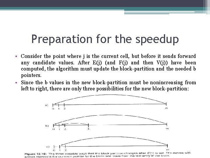
Preparation fοr the speedup • Consider the point where j is the current cell, but before it sends forward any candidate values. After E(j) (and F(j) and then V(j)) have been computed, the algorithm must update the block-partition and the needed b pointers. • Since the b values in the new block-partition must be nonincreasing from left to right, there are only three possibilities for the new block-partition:

Preparation fοr the speedup

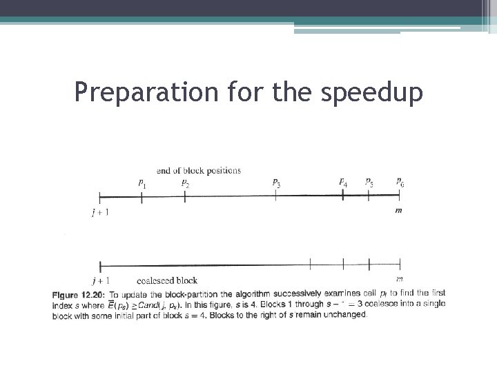
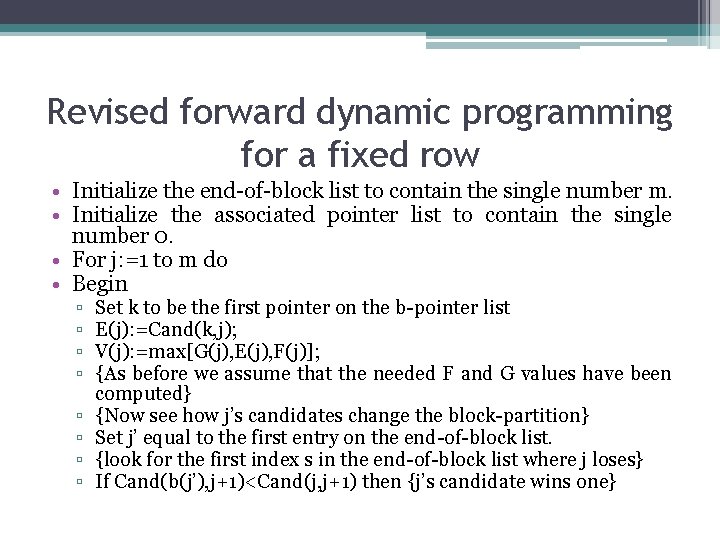
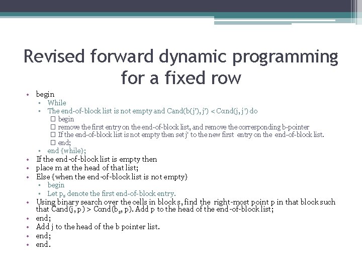
Revised forward dynamic programming for a fixed row • Initialize the end-of-block list to contain the single number m. • Initialize the associated pointer list to contain the single number 0. • For j: =1 to m do • Begin ▫ ▫ ▫ ▫ Set k to be the first pointer on the b-pointer list E(j): =Cand(k, j); V(j): =max[G(j), E(j), F(j)]; {As before we assume that the needed F and G values have been computed} {Now see how j’s candidates change the block-partition} Set j’ equal to the first entry on the end-of-block list. {look for the first index s in the end-of-block list where j loses} If Cand(b(j’), j+1)<Cand(j, j+1) then {j’s candidate wins one}

Revised forward dynamic programming for a fixed row • begin ▫ While ▫ The end-of-block list is not empty and Cand(b(j’), j’) < Cαnd(j, j') do • • � begin � remove the first entry on the end-of-block list, and remove the corresponding b-pointer � If the end-of-block list is not empty then set j' to the new first entry on the end-of-block list. � end; end {while}; ▫ If the end-of-block list is empty then place m at the head of that list; Else {when the end-of-block list is not empty} ▫ begin ▫ Let ps denote the first end-of-block entry. Using binary search over the cells in block s, find the right-most point p in that block such that Cand(j, p) > Cαnd(bs, p). Add p to the head of the end-of-block list; end; Add j to the head of the b pointer list. end; end.

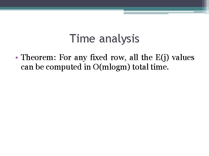
Time analysis • Theorem: For any fixed row, all the E(j) values can be computed in O(mlogm) total time.

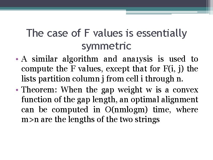
The case of F values is essentially symmetric • A similar algorithm and ana 1 ysis is used to compute the F values, except that for F(i, j) the lists partition column j from cell i through n. • Theorem: When the gap weight w is a convex function of the gap length, an optimal alignment can be computed in O(nmlogm) time, where m>n are the lengths of the two strings

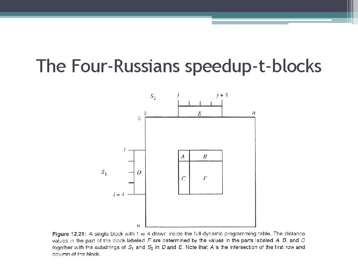
The Four-Russians speedup-t-blocks • Definition: A t-block is a t by t square in the dynamic programming table. • The rough idea of the Four-Russians method is to partition the dynamic programming table into t-blocks and compute the essential values in the table one t-block at a time, rather than one cell at a time. • Lemma: The distance values in a t-block starting in position (i, j) are a function of the values in its first row and column and the substrings S 1[i…i+t-1] and S 2[j. . j+t-1]. • Definition: Given above lemma and the following figure, we define the block function as the function from the five inputs (A, B, C, D, E) to the output F • The values in the last row and column of a r-block are also a function of the inputs (A, Β , C, D, Ε). We call the function from those inputs to the values in the last row and column of a r-block, the restricted block function.

The Four-Russians speedup-t-blocks

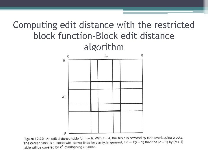
Computing edit distance with the restricted block function–Block edit distance algorithm • Cover the (n+1) by (n+1) dynamic programming table with t-blocks, where the last column of every t-block is shared with the first column of the t-block to its right (if any), and the last row of every tblock is shared with the first row of the t-block below it (if any). In this way, and since n=k(t-1), the table will consist of k rows and k columns of partially overlapping t-blocks. • Initialize the values in the first row and column of the full table according to the base conditions of the recurrence. • In a rowwise manner, use the restricted block function to successively determine the values in the last row and last column of each block. By the overlapping nature of the blocks, the values in the last column (or row) of a block are the values in the first column (or row) of the block to its right (or below it) • The value in cell (n, n) is the edit distance of S 1 and S 2.

Computing edit distance with the restricted block function–Block edit distance algorithm

Accounting detail • block edit distance algorithm ▫ the sizes of the input and the output of the restricted block function are both O(t). There are Θ(n 2/t 2) blocks, hence the total time used by the block edit distance algorithm is o(n 2/t). Setting t to Θ(log n), the time is O(n 2/lοgn). However in the unit-cost RAM model of computation, each output value can be retrieved in constant time since t=O(logn). =>the method is reduced to O(n 2 /(logn)2). • precomputation time ▫ The key issue involves the number of input choices to the restricted block function. ▫ Every cell has an integer from zero to n=>(n+1)t possible values for any t-length row or column. ▫ If the alphabet has size σ, then there are σt, possible substrings of length t=>#distinct input combinations to the restricted block function: is (n + 1)2 t σ2 t ▫ For each input, it takes Θ(t 2) time to evaluate the last row and column of the resulting r-block (by running the standard dynamic program). Thus the overall time used in this way to precompute the function outputs to all possible input choices is Θ((n + 1)2 t σ2 tt 2).

The trick: offset encoding • Lemma: In any row, column, or diagonal of the dynamic programming table for edit distance, two adjacent cells can have a value that differs by at most one. • Definition: The offset vector is a t-length vector of values from {1, 0, 1}, where the first entry must be zero. • Theorem: Consider a t-block with upper left corner in position (i, j). The two offset vectors for the last row and last column of the block can be determined from the two offset vectors for the first row and column of the block and from substrings S 1[1. . i] and S 2[1. . j]. That is, no D value is needed in the input in order to determine the offset vectors in the last row and column of the block. • Definition: The function that determines the two offset vectors for the last row and last column from the two offset vectors for the first row and column of a block together with substrings S 1[1. . i] and S 2[1. . j] is called the offset function

Four-Russians edit distance algorithm • Cover the n by n dynamic programming table with t-blocks, where the last column of every t-block is shared with the first column of the t-block to its right (if any), and the last row of every t-block is shared with the first row of the t-block below it (if any) • Initialize the values in the first row and column of the full table according to the base conditions of the recurrence. Compute the offset values in the first row and column. • In a rowwise manner, use the offset block function to successively determine the offset vectors of the last row and column of each block. By the overlapping nature of the blocks, the offset vector in the last column (or row) of a block provides the next offset vector in the entry in the next vector to zero • Let Q be the total of the offset values computed for cells in row n. D(n, n) = D(n, 0)+Q =n +Q

Time analysis • Theorem: The edit distance of two strings of length n can be computed in O(n 2/logn) time or O(n 2/(logn)2) time in the unit-cost RAM model