REFINERY OPERATIONS PLANNING Dunham Luhila Odunuga Overview Refinery

REFINERY OPERATIONS PLANNING Dunham, Luhila, Odunuga

Overview Refinery Overview Production Planning Linear model with complex and simplified utilities Results Conclusions

Model Refinery: Bangchak Refinery (Thailand)

What is Refinery Operations Planning? q How much crude should be purchased? q What kind/quality of crude should be purchased? q How much does the refinery want to produce? Consists of crude oil unloading, production planning and distribution q

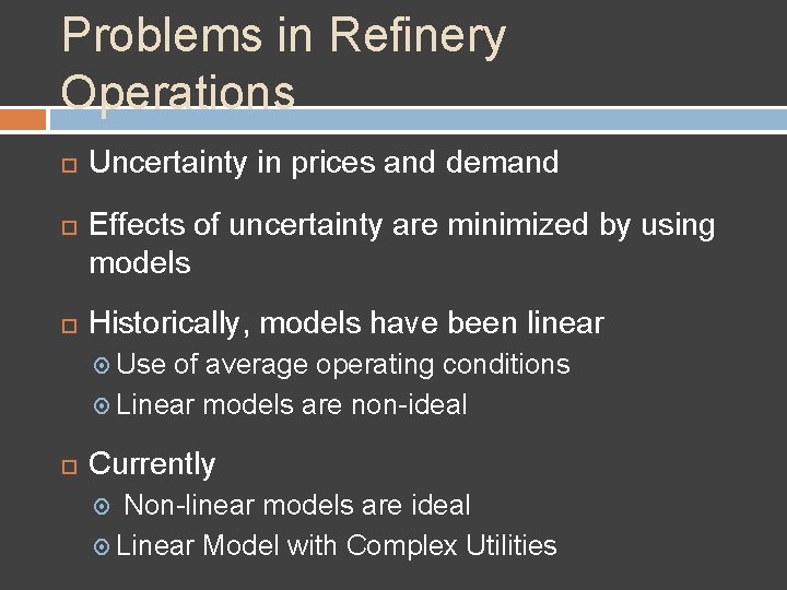
Problems in Refinery Operations Uncertainty in prices and demand Effects of uncertainty are minimized by using models Historically, models have been linear Use of average operating conditions Linear models are non-ideal Currently Non-linear models are ideal Linear Model with Complex Utilities

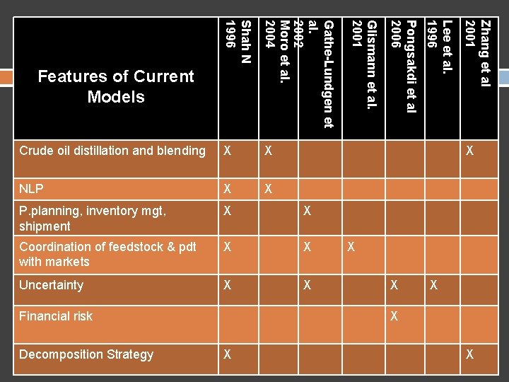
X X P. planning, inventory mgt, shipment X X Coordination of feedstock & pdt with markets X X Uncertainty X X Financial risk Decomposition Strategy Zhang et al 2001 NLP Lee et al. 1996 X Pongsakdi et al 2006 Gathe-Lundgen et al. 2002 Moro et al. 2004 X Glismann et al. 2001 Shah N 1996 Crude oil distillation and blending Features of Current Models X X X X

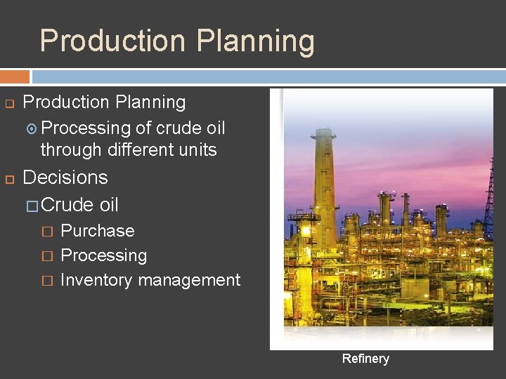
Production Planning q Production Planning Processing of crude oil through different units Decisions � Crude oil � � � Purchase Processing Inventory management Bangchak Refinery

Production Planning Routine process which guides purchasing Departments Crude oil acquisition, product sales & refinery operations Based on Market demands and prices Uncertainty

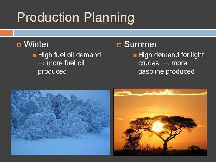
Production Planning Winter High fuel oil demand → more fuel oil produced Summer High demand for light crudes → more gasoline produced

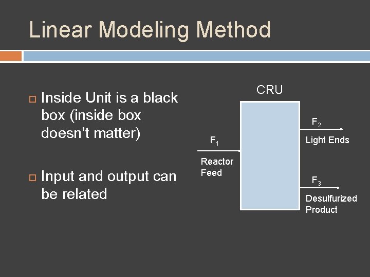
Linear Modeling Method Inside Unit is a black box (inside box doesn’t matter) Input and output can be related CRU F 2 F 1 Reactor Feed Light Ends F 3 Desulfurized Product

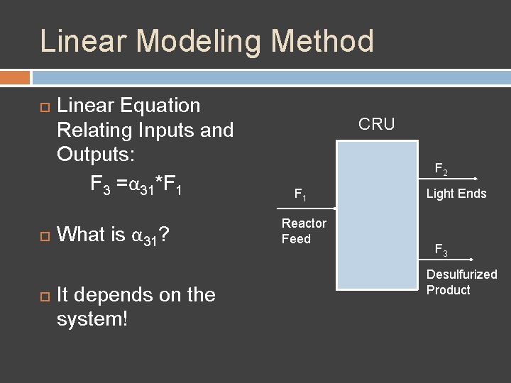
Linear Modeling Method Linear Equation Relating Inputs and Outputs: F 3 =α 31*F 1 What is α 31? It depends on the system! CRU F 2 F 1 Reactor Feed Light Ends F 3 Desulfurized Product

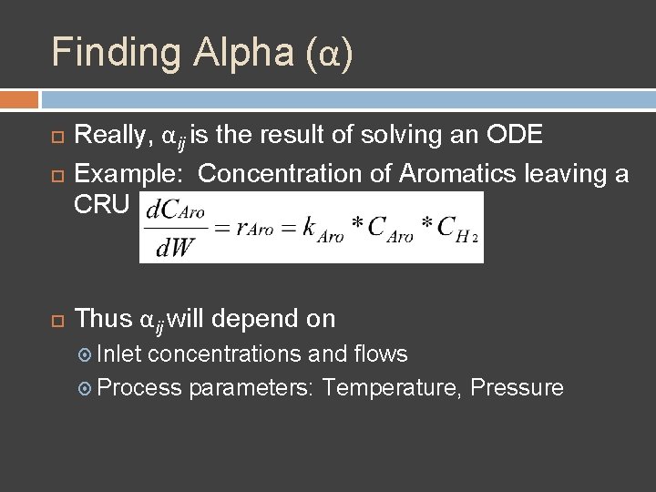
Finding Alpha (α) Really, αij is the result of solving an ODE Example: Concentration of Aromatics leaving a CRU Thus αij will depend on Inlet concentrations and flows Process parameters: Temperature, Pressure

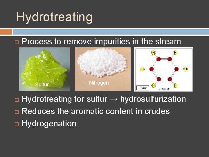
Hydrotreating Process to remove impurities in the stream Aromatics Sulfur Nitrogen Hydrotreating for sulfur → hydrosulfurization Reduces the aromatic content in crudes Hydrogenation

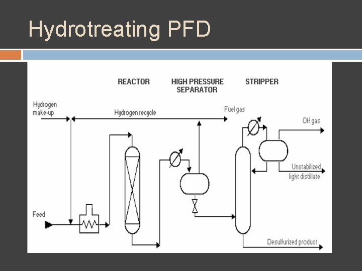
Hydrotreating PFD

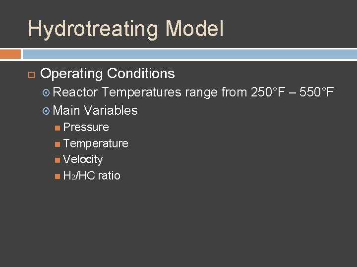
Hydrotreating Model Operating Conditions Reactor Temperatures range from 250°F – 550°F Main Variables Pressure Temperature Velocity H 2/HC ratio

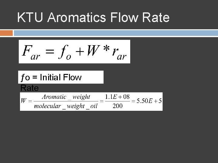
KTU Aromatics Flow Rate ƒo = Initial Flow Rate

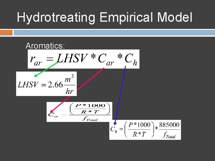
Hydrotreating Empirical Model Aromatics:

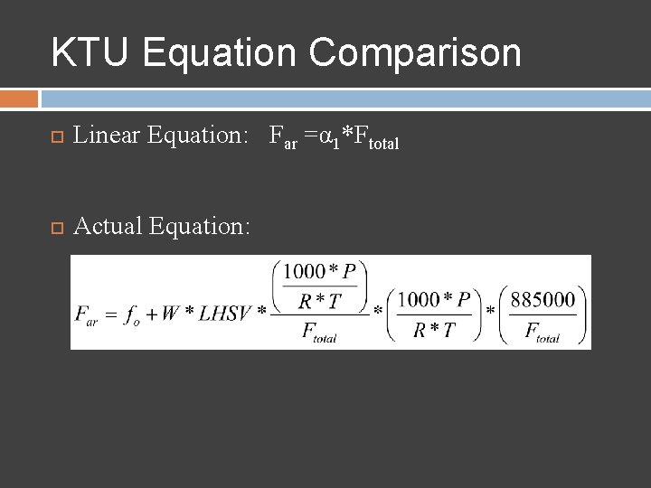
KTU Equation Comparison Linear Equation: Far =α 1*Ftotal Actual Equation:

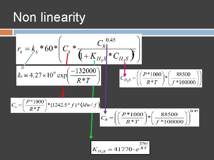
Non linearity

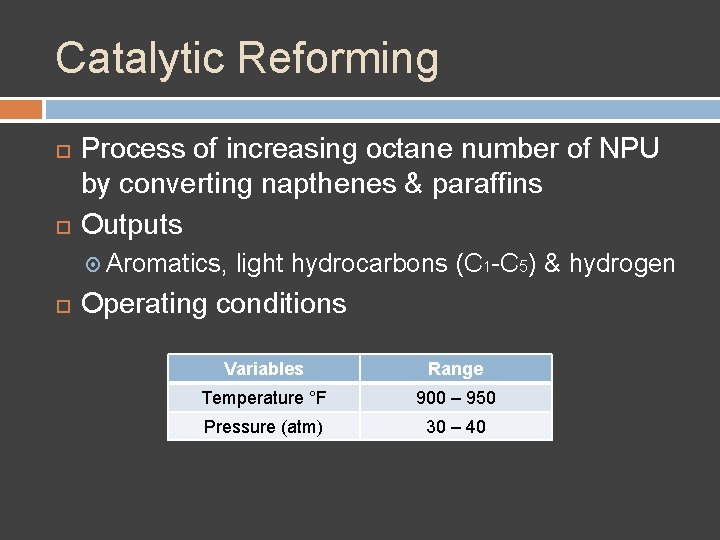
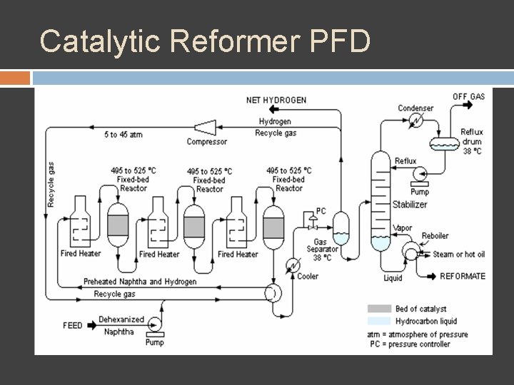
Catalytic Reforming Process of increasing octane number of NPU by converting napthenes & paraffins Outputs Aromatics, light hydrocarbons (C 1 -C 5) & hydrogen Operating conditions Variables Range Temperature °F 900 – 950 Pressure (atm) 30 – 40

Catalytic Reformer PFD

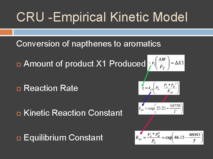
CRU -Empirical Kinetic Model Conversion of napthenes to aromatics Amount of product X 1 Produced Reaction Rate Kinetic Reaction Constant Equilibrium Constant

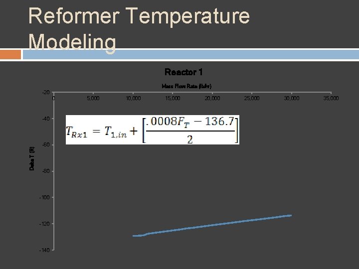
Reformer Temperature Modeling Reactor 1 Mass Flow Rate (lb/hr) -20 0 Delta T (R) -40 -60 -80 -100 -120 -140 5, 000 10, 000 15, 000 20, 000 25, 000 30, 000 35, 000

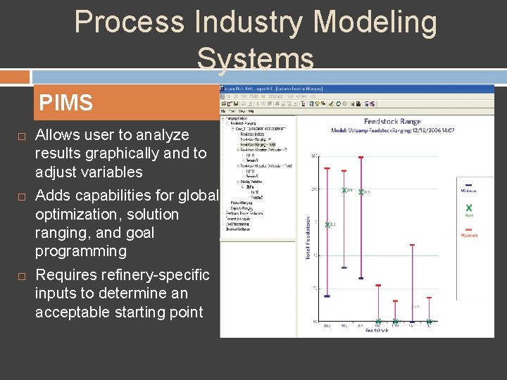
Process Industry Modeling Systems PIMS Allows user to analyze results graphically and to adjust variables Adds capabilities for global optimization, solution ranging, and goal programming Requires refinery-specific inputs to determine an acceptable starting point

PIMS and Non-linearities Benefits Identifies the solution that maximizes global profitability Validates solution and enhances planners’ confidence and gives an estimate on how close results are to optimal solution Eliminates solutions need to manually search for improved

PIMS and Non-linearities SLP is the primary non-linear modeling feature Flexibility in the types of equations that can be used in models Builds derivatives which eliminates potential errors Non-linear terms can reference existing Aspen PIMs variables or define new variables

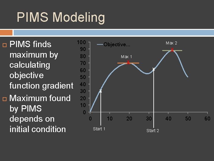
PIMS Modeling PIMS finds maximum by calculating objective function gradient Maximum found by PIMS depends on initial condition 100 90 80 70 60 50 40 30 20 10 0 Max 2 Objective. . . X Max 1 X x x 0 10 Start 1 20 30 Start 2 40 50 60

Alternative Method Linear Model with Utilities

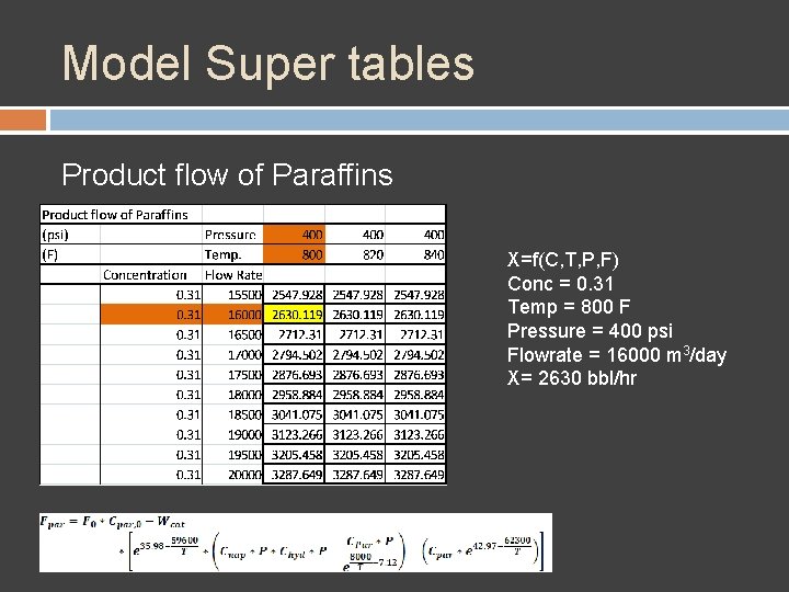
Model Super tables Product flow of Paraffins X=f(C, T, P, F) Conc = 0. 31 Temp = 800 F Pressure = 400 psi Flowrate = 16000 m 3/day X= 2630 bbl/hr

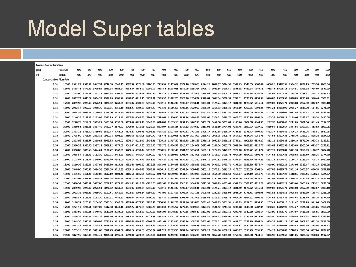
Model Super tables

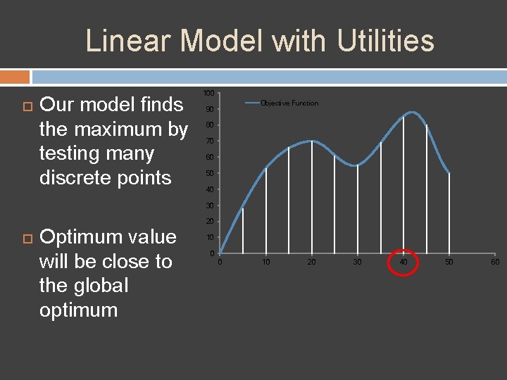
Linear Model with Utilities Our model finds the maximum by testing many discrete points 100 Objective Function 90 80 70 60 50 40 30 Optimum value will be close to the global optimum 20 10 0 0 10 20 30 40 50 60

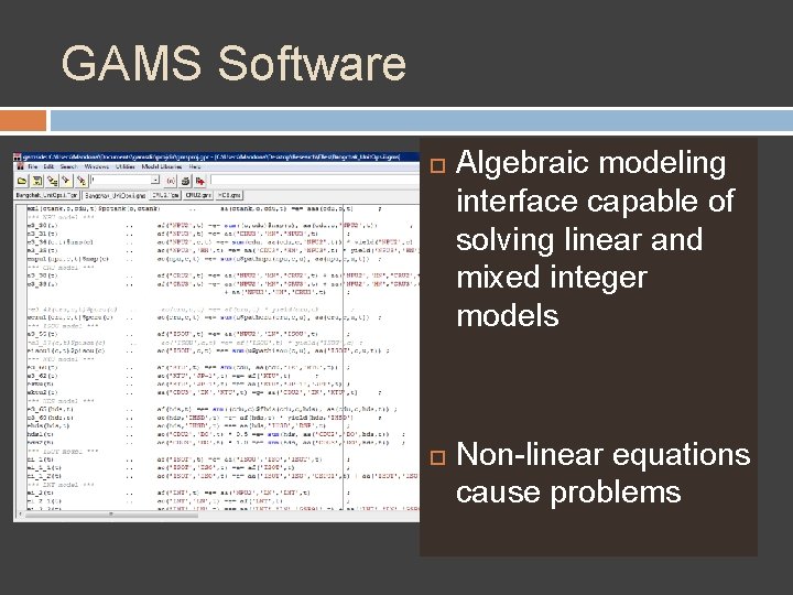
GAMS Software Algebraic modeling interface capable of solving linear and mixed integer models Non-linear equations cause problems

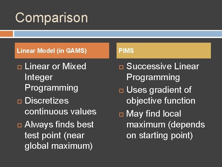
Comparison Linear Model (in GAMS) Linear or Mixed Integer Programming Discretizes continuous values Always finds best test point (near global maximum) PIMS Successive Linear Programming Uses gradient of objective function May find local maximum (depends on starting point)

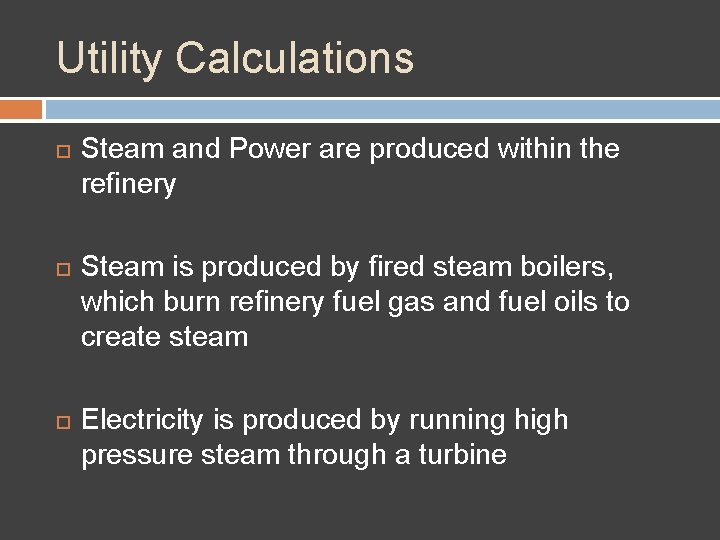
Utility Calculations Steam and Power are produced within the refinery Steam is produced by fired steam boilers, which burn refinery fuel gas and fuel oils to create steam Electricity is produced by running high pressure steam through a turbine

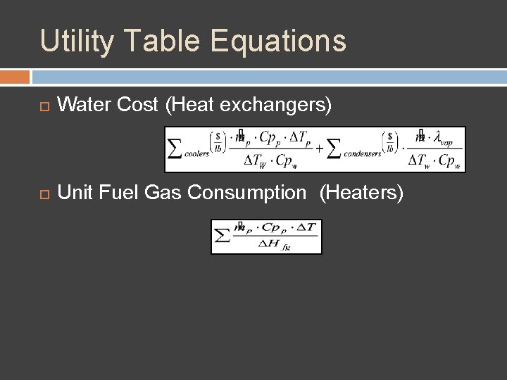
Utility Table Equations Water Cost (Heat exchangers) Unit Fuel Gas Consumption (Heaters)

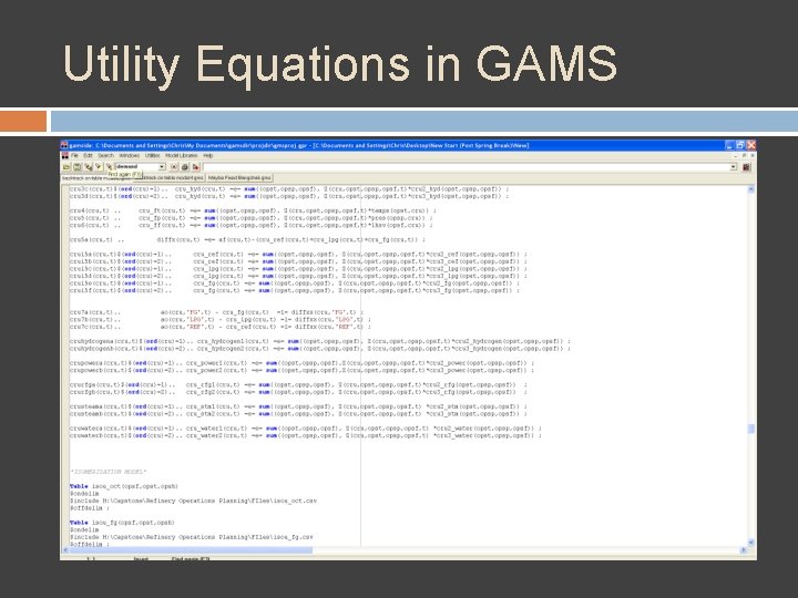
Utility Equations in GAMS

Results

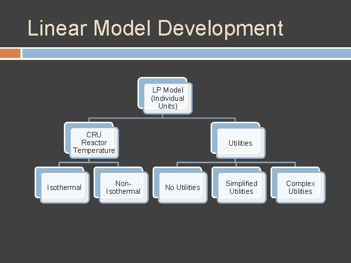
Linear Model Development LP Model (Individual Units) CRU Reactor Temperature Isothermal Non. Isothermal Utilities No Utilities Simplified Utilities Complex Utilities

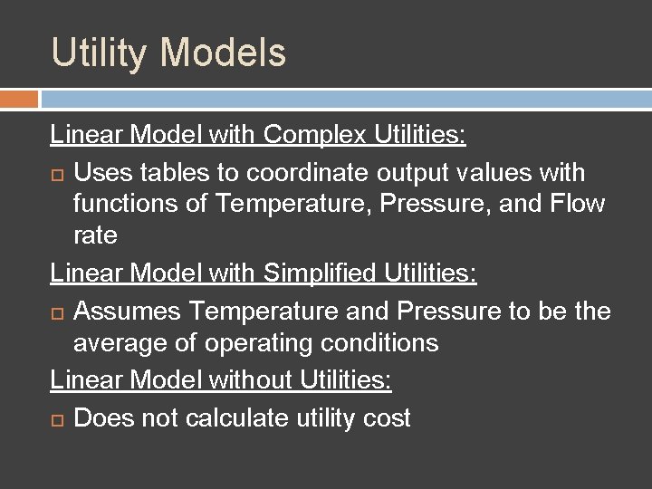
Utility Models Linear Model with Complex Utilities: Uses tables to coordinate output values with functions of Temperature, Pressure, and Flow rate Linear Model with Simplified Utilities: Assumes Temperature and Pressure to be the average of operating conditions Linear Model without Utilities: Does not calculate utility cost

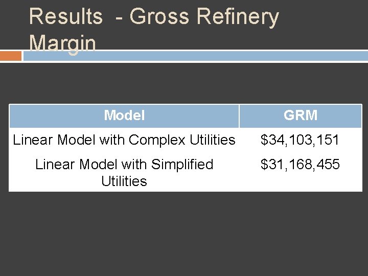
Results - Gross Refinery Margin Model GRM Linear Model with Complex Utilities $34, 103, 151 Linear Model with Simplified Utilities $31, 168, 455

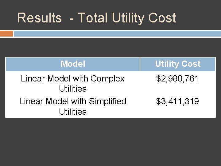
Results - Total Utility Cost Model Utility Cost Linear Model with Complex Utilities Linear Model with Simplified Utilities $2, 980, 761 $3, 411, 319

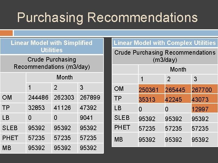
Purchasing Recommendations Linear Model with Simplified Utilities Crude Purchasing Recommendations (m 3/day) Linear Model with Complex Utilities Crude Purchasing Recommendations (m 3/day) Month 1 2 1 3 2 3 OM 250361 265445 267700 OM 244486 262303 267899 TP 35313 42245 43073 TP 32853 41126 47392 LB 0 0 12997 LB 0 0 9041 SLEB 95392 95392 PHET 57235 57235 MB 95392 95392

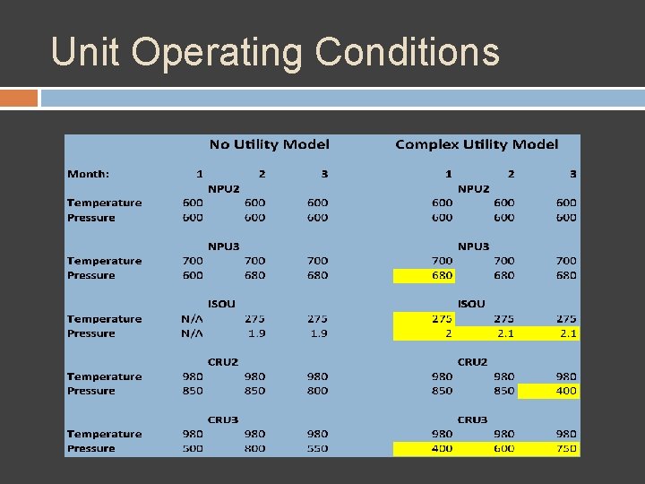
Unit Operating Conditions

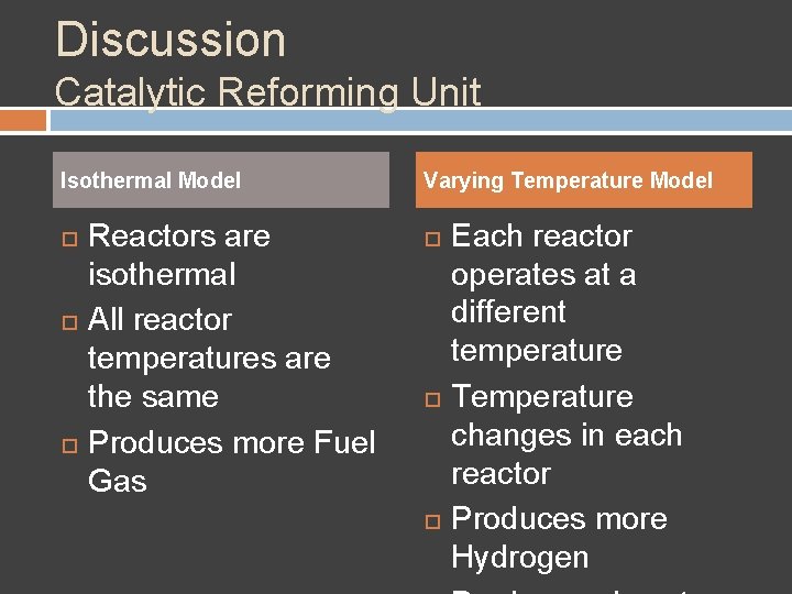
Discussion Catalytic Reforming Unit Isothermal Model Reactors are isothermal All reactor temperatures are the same Produces more Fuel Gas Varying Temperature Model Each reactor operates at a different temperature Temperature changes in each reactor Produces more Hydrogen

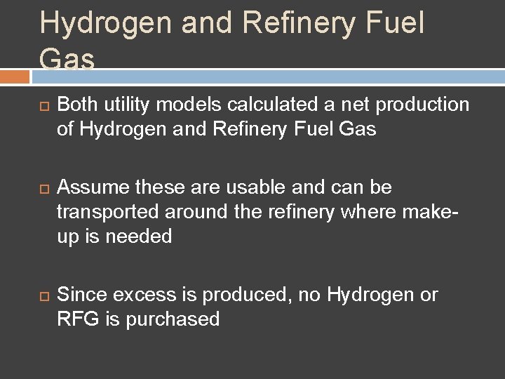
Hydrogen and Refinery Fuel Gas Both utility models calculated a net production of Hydrogen and Refinery Fuel Gas Assume these are usable and can be transported around the refinery where makeup is needed Since excess is produced, no Hydrogen or RFG is purchased

Conclusions The Linear Model with Complex Utilities processes more crude and gives a larger GRM than a model with Simplified Utilities and a model with no utility cost calculation The Non-isothermal CRU model produces more reformate and increases overall GRM Linear models in GAMS always find a value close to the global optimum, where PIMS may find only a local optimum depending on

Questions?