Recursive algorithms n Recursive solution solve a smaller

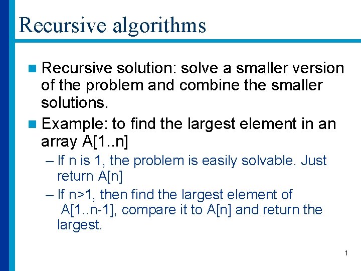
Recursive algorithms n Recursive solution: solve a smaller version of the problem and combine the smaller solutions. n Example: to find the largest element in an array A[1. . n] – If n is 1, the problem is easily solvable. Just return A[n] – If n>1, then find the largest element of A[1. . n-1], compare it to A[n] and return the largest. 1

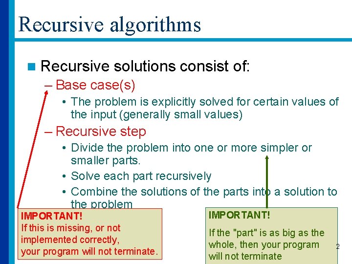
Recursive algorithms n Recursive solutions consist of: – Base case(s) • The problem is explicitly solved for certain values of the input (generally small values) – Recursive step • Divide the problem into one or more simpler or smaller parts. • Solve each part recursively • Combine the solutions of the parts into a solution to the problem IMPORTANT! If this is missing, or not implemented correctly, your program will not terminate. IMPORTANT! If the "part" is as big as the whole, then your program will not terminate 2

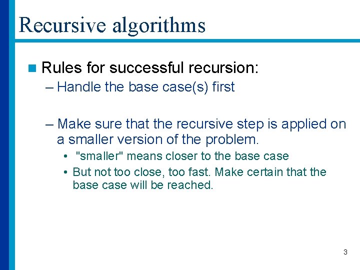
Recursive algorithms n Rules for successful recursion: – Handle the base case(s) first – Make sure that the recursive step is applied on a smaller version of the problem. • "smaller" means closer to the base case • But not too close, too fast. Make certain that the base case will be reached. 3

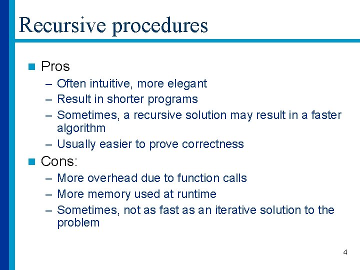
Recursive procedures n Pros – Often intuitive, more elegant – Result in shorter programs – Sometimes, a recursive solution may result in a faster algorithm – Usually easier to prove correctness n Cons: – More overhead due to function calls – More memory used at runtime – Sometimes, not as fast as an iterative solution to the problem 4

Recursive procedures Any problem that can be solved recursively can be solved iteratively n Choose recursion when n – you have a recursive data structure – the recursive solution is easier to understand/debug n Do not choose recursion when – performance is an issue n Examples where recursion is better – Towers of Hanoi, certain sorting algorithms 5

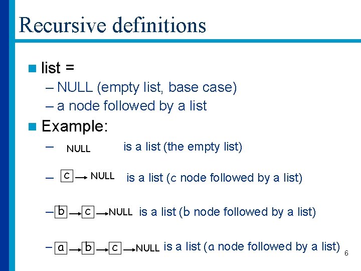
Recursive definitions n list = – NULL (empty list, base case) – a node followed by a list n Example: – is a list (the empty list) NULL – c NULL –b c – a b is a list (c node followed by a list) NULL c is a list (b node followed by a list) NULL is a list (a node followed by a list) 6

Time Analysis n. A recursive algorithm contains a call to itself. n Computing the running time of a recursive algorithm involves solving a recurrence equation: one that describes the running time in a recursive manner. n We will describe the process through an example 7

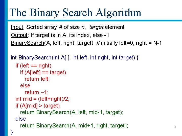
The Binary Search Algorithm Input: Sorted array A of size n, target element Output: If target is in A, its index, else -1 Binary. Search(A, left, right, target) // initially left=0, right = N-1 int Binary. Search(int A[ ], int left, int right, int target) { if (left == right) if (A[left] == target) return left; else return – 1; int mid = (left+right)/2; if (A[mid] > target) return Binary. Search(A, left, mid-1, target); else return Binary. Search(A, mid+1, right, target); } 8

The Binary Search Algorithm int Binary. Search(int A[ ], int left, int right, int target) { if (left == right) if (A[left] == target) return left; Constant time operations. else Their duration is always the same return – 1; regardless of n's value. int mid = (left+right)/2; if (A[mid] > target) return Binary. Search(A, left, mid-1, target); else return Binary. Search(A, mid+1, right, target); } How long would this take? 9

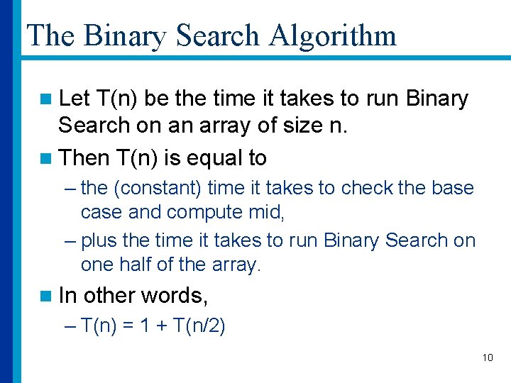
The Binary Search Algorithm n Let T(n) be the time it takes to run Binary Search on an array of size n. n Then T(n) is equal to – the (constant) time it takes to check the base case and compute mid, – plus the time it takes to run Binary Search on one half of the array. n In other words, – T(n) = 1 + T(n/2) 10

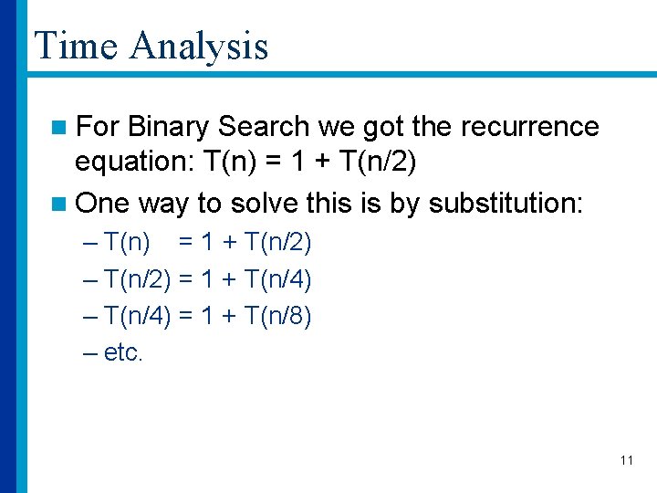
Time Analysis n For Binary Search we got the recurrence equation: T(n) = 1 + T(n/2) n One way to solve this is by substitution: – T(n) = 1 + T(n/2) – T(n/2) = 1 + T(n/4) – T(n/4) = 1 + T(n/8) – etc. 11

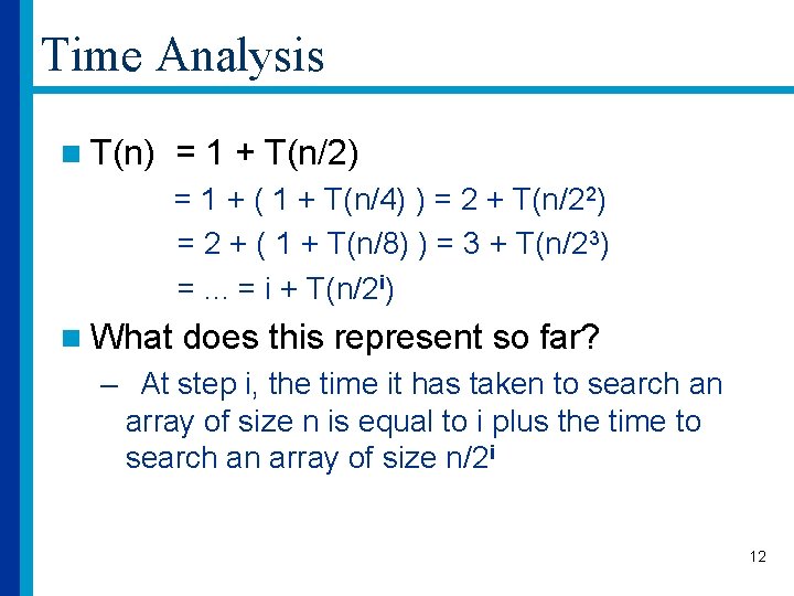
Time Analysis n T(n) = 1 + T(n/2) = 1 + ( 1 + T(n/4) ) = 2 + T(n/22) = 2 + ( 1 + T(n/8) ) = 3 + T(n/23) =. . . = i + T(n/2 i) n What does this represent so far? – At step i, the time it has taken to search an array of size n is equal to i plus the time to search an array of size n/2 i 12

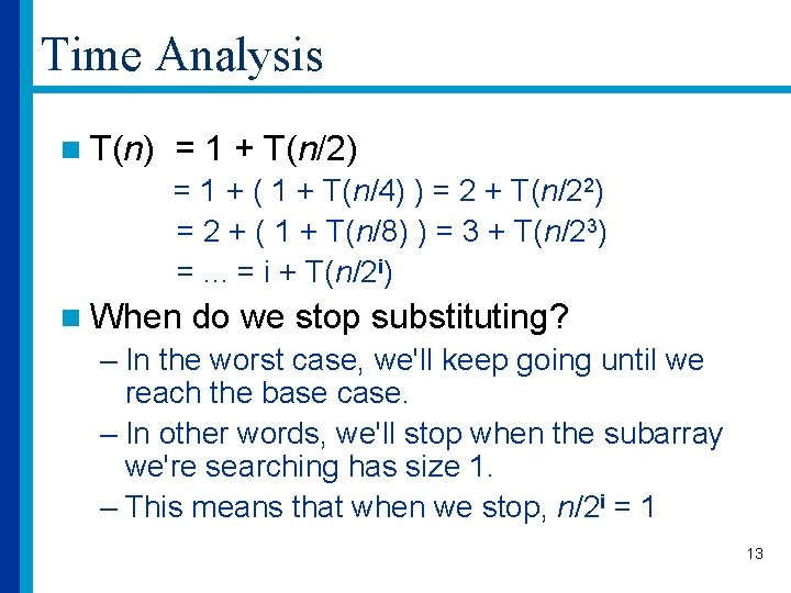
Time Analysis n T(n) = 1 + T(n/2) = 1 + ( 1 + T(n/4) ) = 2 + T(n/22) = 2 + ( 1 + T(n/8) ) = 3 + T(n/23) =. . . = i + T(n/2 i) n When do we stop substituting? – In the worst case, we'll keep going until we reach the base case. – In other words, we'll stop when the subarray we're searching has size 1. – This means that when we stop, n/2 i = 1 13

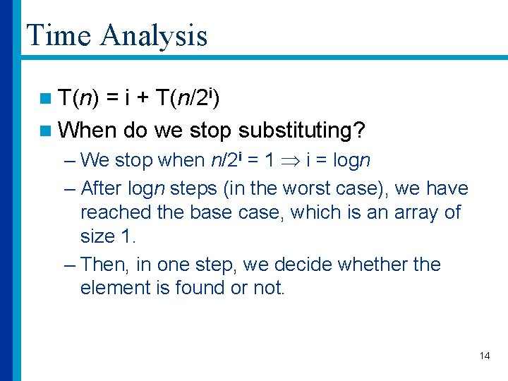
Time Analysis n T(n) = i + T(n/2 i) n When do we stop substituting? – We stop when n/2 i = 1 i = logn – After logn steps (in the worst case), we have reached the base case, which is an array of size 1. – Then, in one step, we decide whether the element is found or not. 14

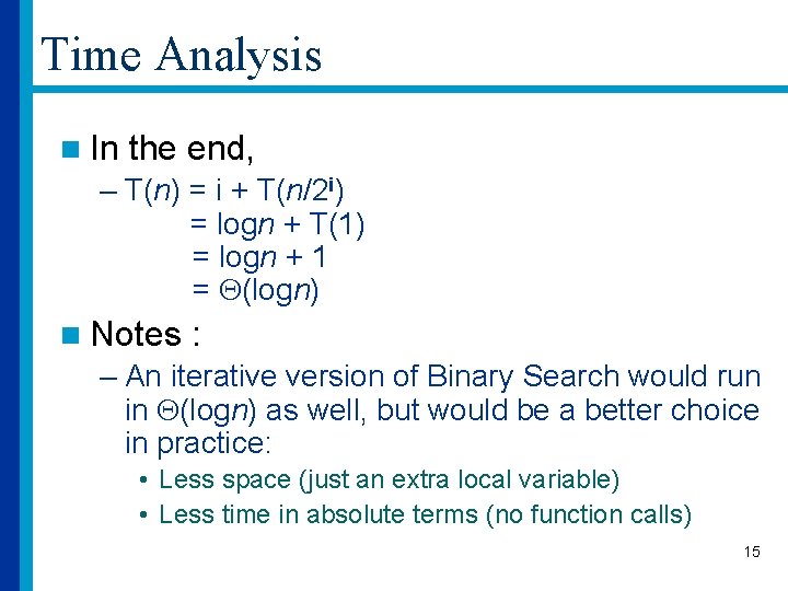
Time Analysis n In the end, – T(n) = i + T(n/2 i) = logn + T(1) = logn + 1 = (logn) n Notes : – An iterative version of Binary Search would run in (logn) as well, but would be a better choice in practice: • Less space (just an extra local variable) • Less time in absolute terms (no function calls) 15