Recursion and Dynamic Programming CSE 2320 Algorithms and

Recursion and Dynamic Programming CSE 2320 – Algorithms and Data Structures Vassilis Athitsos University of Texas at Arlington 1

Recursion • Recursion is a fundamental concept in computer science. • Recursive algorithms: algorithms that solve a problem by solving one or more smaller instances of the same problem. • Recursive functions: functions that call themselves. • Recursive data types: data types that are defined using references to themselves. • Example? 2

Recursion • Recursion is a fundamental concept in computer science. • Recursive algorithms: algorithms that solve a problem by solving one or more smaller instances of the same problem. • Recursive functions: functions that call themselves. • Recursive data types: data types that are defined using references to themselves. • Example? Nodes in the implementation of linked lists. • In all recursive concepts, there is one or more base cases. No recursive concept can be understood without understanding its base cases. • What is the base case for nodes? 3

Recursion • Recursion is a fundamental concept in computer science. • Recursive algorithms: algorithms that solve a problem by solving one or more smaller instances of the same problem. • Recursive functions: functions that call themselves. • Recursive data types: data types that are defined using references to themselves. • Example? Nodes in the implementation of linked lists. • In all recursive concepts, there is one or more base cases. No recursive concept can be understood without understanding its base cases. • What is the base case for nodes? – A node pointing to NULL. 4

Recursive Algorithms • Recursive algorithms: algorithms that solve a problem by solving one or more smaller instances of the same problem. • A recursive algorithm can always be implemented both using recursive functions, and without recursive functions. • Example of a recursive function: 5

Recursive Algorithms • Recursive algorithms: algorithms that solve a problem by solving one or more smaller instances of the same problem. • A recursive algorithm can always be implemented both using recursive functions, and without recursive functions. • Example of a recursive function: the factorial. – Recursive definition? – Non-recursive definition? 6

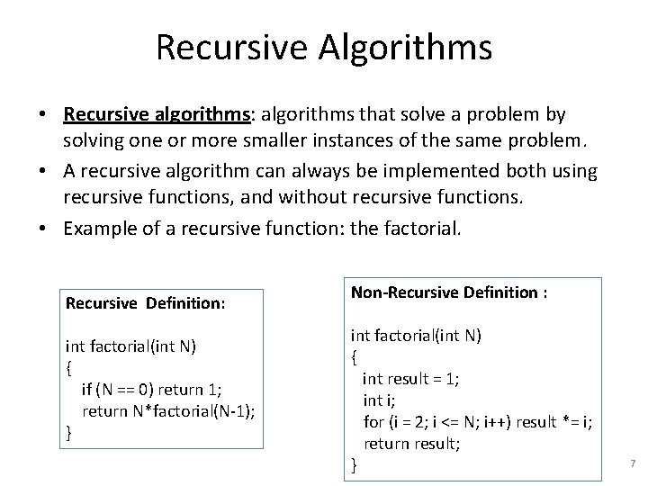
Recursive Algorithms • Recursive algorithms: algorithms that solve a problem by solving one or more smaller instances of the same problem. • A recursive algorithm can always be implemented both using recursive functions, and without recursive functions. • Example of a recursive function: the factorial. Recursive Definition: int factorial(int N) { if (N == 0) return 1; return N*factorial(N-1); } Non-Recursive Definition : int factorial(int N) { int result = 1; int i; for (i = 2; i <= N; i++) result *= i; return result; } 7

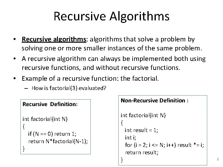
Recursive Algorithms • Recursive algorithms: algorithms that solve a problem by solving one or more smaller instances of the same problem. • A recursive algorithm can always be implemented both using recursive functions, and without recursive functions. • Example of a recursive function: the factorial. – How is factorial(3) evaluated? Recursive Definition: int factorial(int N) { if (N == 0) return 1; return N*factorial(N-1); } Non-Recursive Definition : int factorial(int N) { int result = 1; int i; for (i = 2; i <= N; i++) result *= i; return result; } 8

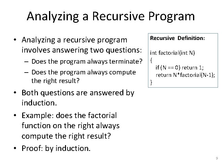
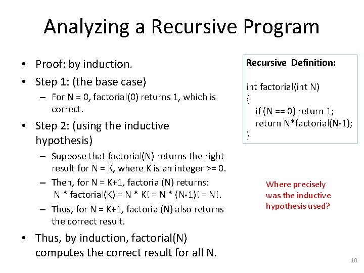
Analyzing a Recursive Program • Analyzing a recursive program involves answering two questions: – Does the program always terminate? – Does the program always compute the right result? Recursive Definition: int factorial(int N) { if (N == 0) return 1; return N*factorial(N-1); } • Both questions are answered by induction. • Example: does the factorial function on the right always compute the right result? • Proof: by induction. 9

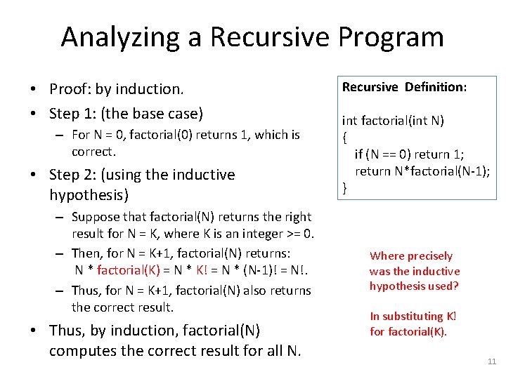
Analyzing a Recursive Program • Proof: by induction. • Step 1: (the base case) – For N = 0, factorial(0) returns 1, which is correct. • Step 2: (using the inductive hypothesis) – Suppose that factorial(N) returns the right result for N = K, where K is an integer >= 0. – Then, for N = K+1, factorial(N) returns: N * factorial(K) = N * K! = N * (N-1)! = N!. – Thus, for N = K+1, factorial(N) also returns the correct result. • Thus, by induction, factorial(N) computes the correct result for all N. Recursive Definition: int factorial(int N) { if (N == 0) return 1; return N*factorial(N-1); } Where precisely was the inductive hypothesis used? 10

Analyzing a Recursive Program • Proof: by induction. • Step 1: (the base case) – For N = 0, factorial(0) returns 1, which is correct. • Step 2: (using the inductive hypothesis) – Suppose that factorial(N) returns the right result for N = K, where K is an integer >= 0. – Then, for N = K+1, factorial(N) returns: N * factorial(K) = N * K! = N * (N-1)! = N!. – Thus, for N = K+1, factorial(N) also returns the correct result. • Thus, by induction, factorial(N) computes the correct result for all N. Recursive Definition: int factorial(int N) { if (N == 0) return 1; return N*factorial(N-1); } Where precisely was the inductive hypothesis used? In substituting K! for factorial(K). 11

Guidelines for Designing Recursive Functions • We should design recursive functions so that it is easy to convince ourselves that they are correct. – Strictly speaking, the only way to convince ourselves is a mathematical proof. – Loosely speaking, we should follow some guidelines to make our life easier. • So, it is a good idea for our recursive functions to follow these rules: – They must explicitly solve one or more base cases. – Each recursive call must involve smaller values of the arguments, or smaller sizes of the problem. 12

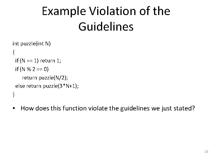
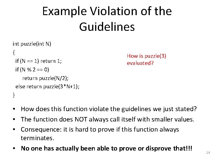
Example Violation of the Guidelines int puzzle(int N) { if (N == 1) return 1; if (N % 2 == 0) return puzzle(N/2); else return puzzle(3*N+1); } • How does this function violate the guidelines we just stated? 13

Example Violation of the Guidelines int puzzle(int N) { if (N == 1) return 1; if (N % 2 == 0) return puzzle(N/2); else return puzzle(3*N+1); } How is puzzle(3) evaluated? • How does this function violate the guidelines we just stated? • The function does NOT always call itself with smaller values. • Consequence: it is hard to prove if this function always terminates. • No one has actually been able to prove or disprove that!!! 14

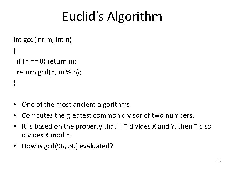
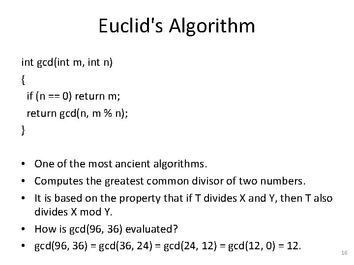
Euclid's Algorithm int gcd(int m, int n) { if (n == 0) return m; return gcd(n, m % n); } • One of the most ancient algorithms. • Computes the greatest common divisor of two numbers. • It is based on the property that if T divides X and Y, then T also divides X mod Y. • How is gcd(96, 36) evaluated? 15

Euclid's Algorithm int gcd(int m, int n) { if (n == 0) return m; return gcd(n, m % n); } • One of the most ancient algorithms. • Computes the greatest common divisor of two numbers. • It is based on the property that if T divides X and Y, then T also divides X mod Y. • How is gcd(96, 36) evaluated? • gcd(96, 36) = gcd(36, 24) = gcd(24, 12) = gcd(12, 0) = 12. 16

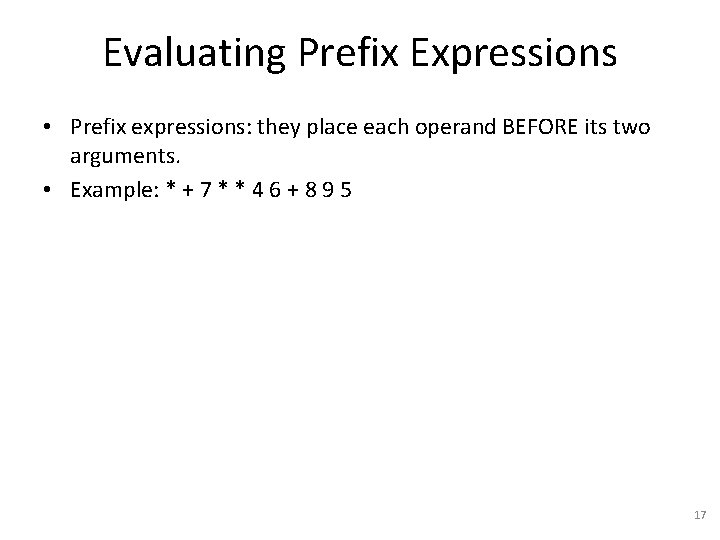
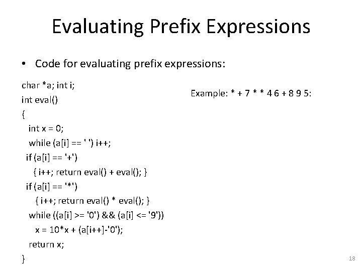
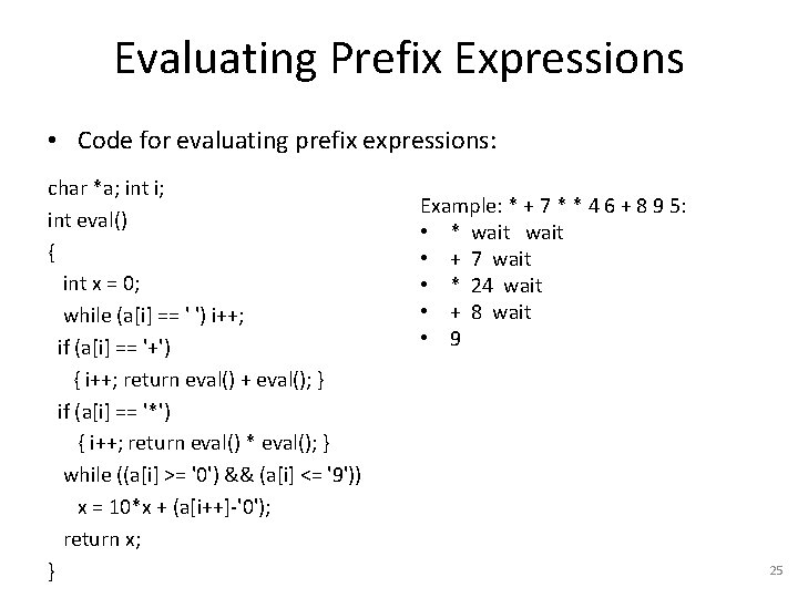
Evaluating Prefix Expressions • Prefix expressions: they place each operand BEFORE its two arguments. • Example: * + 7 * * 4 6 + 8 9 5 17

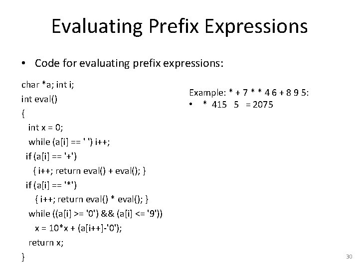
Evaluating Prefix Expressions • Code for evaluating prefix expressions: char *a; int i; int eval() { int x = 0; while (a[i] == ' ') i++; if (a[i] == '+') { i++; return eval() + eval(); } if (a[i] == '*') { i++; return eval() * eval(); } while ((a[i] >= '0') && (a[i] <= '9')) x = 10*x + (a[i++]-'0'); return x; } Example: * + 7 * * 4 6 + 8 9 5: 18

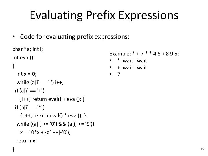
Evaluating Prefix Expressions • Code for evaluating prefix expressions: char *a; int i; int eval() { int x = 0; while (a[i] == ' ') i++; if (a[i] == '+') { i++; return eval() + eval(); } if (a[i] == '*') { i++; return eval() * eval(); } while ((a[i] >= '0') && (a[i] <= '9')) x = 10*x + (a[i++]-'0'); return x; } Example: * + 7 * * 4 6 + 8 9 5: • * wait • + wait • 7 19

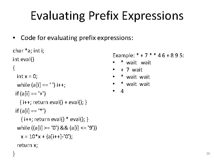
Evaluating Prefix Expressions • Code for evaluating prefix expressions: char *a; int i; int eval() { int x = 0; while (a[i] == ' ') i++; if (a[i] == '+') { i++; return eval() + eval(); } if (a[i] == '*') { i++; return eval() * eval(); } while ((a[i] >= '0') && (a[i] <= '9')) x = 10*x + (a[i++]-'0'); return x; } Example: * + 7 * * 4 6 + 8 9 5: • * wait • + 7 wait • * wait • 4 20

Evaluating Prefix Expressions • Code for evaluating prefix expressions: char *a; int i; int eval() { int x = 0; while (a[i] == ' ') i++; if (a[i] == '+') { i++; return eval() + eval(); } if (a[i] == '*') { i++; return eval() * eval(); } while ((a[i] >= '0') && (a[i] <= '9')) x = 10*x + (a[i++]-'0'); return x; } Example: * + 7 * * 4 6 + 8 9 5: • * wait • + 7 wait • * 4 wait • 6 21

Evaluating Prefix Expressions • Code for evaluating prefix expressions: char *a; int i; int eval() { int x = 0; while (a[i] == ' ') i++; if (a[i] == '+') { i++; return eval() + eval(); } if (a[i] == '*') { i++; return eval() * eval(); } while ((a[i] >= '0') && (a[i] <= '9')) x = 10*x + (a[i++]-'0'); return x; } Example: * + 7 * * 4 6 + 8 9 5: • * wait • + 7 wait • * 4 6 = 24 22

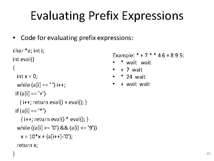
Evaluating Prefix Expressions • Code for evaluating prefix expressions: char *a; int i; int eval() { int x = 0; while (a[i] == ' ') i++; if (a[i] == '+') { i++; return eval() + eval(); } if (a[i] == '*') { i++; return eval() * eval(); } while ((a[i] >= '0') && (a[i] <= '9')) x = 10*x + (a[i++]-'0'); return x; } Example: * + 7 * * 4 6 + 8 9 5: • * wait • + 7 wait • * 24 wait • + wait 23

Evaluating Prefix Expressions • Code for evaluating prefix expressions: char *a; int i; int eval() { int x = 0; while (a[i] == ' ') i++; if (a[i] == '+') { i++; return eval() + eval(); } if (a[i] == '*') { i++; return eval() * eval(); } while ((a[i] >= '0') && (a[i] <= '9')) x = 10*x + (a[i++]-'0'); return x; } Example: * + 7 * * 4 6 + 8 9 5: • * wait • + 7 wait • * 24 wait • + wait • 8 24

Evaluating Prefix Expressions • Code for evaluating prefix expressions: char *a; int i; int eval() { int x = 0; while (a[i] == ' ') i++; if (a[i] == '+') { i++; return eval() + eval(); } if (a[i] == '*') { i++; return eval() * eval(); } while ((a[i] >= '0') && (a[i] <= '9')) x = 10*x + (a[i++]-'0'); return x; } Example: * + 7 * * 4 6 + 8 9 5: • * wait • + 7 wait • * 24 wait • + 8 wait • 9 25

Evaluating Prefix Expressions • Code for evaluating prefix expressions: char *a; int i; int eval() { int x = 0; while (a[i] == ' ') i++; if (a[i] == '+') { i++; return eval() + eval(); } if (a[i] == '*') { i++; return eval() * eval(); } while ((a[i] >= '0') && (a[i] <= '9')) x = 10*x + (a[i++]-'0'); return x; } Example: * + 7 * * 4 6 + 8 9 5: • * wait • + 7 wait • * 24 wait • + 8 9 = 17 26

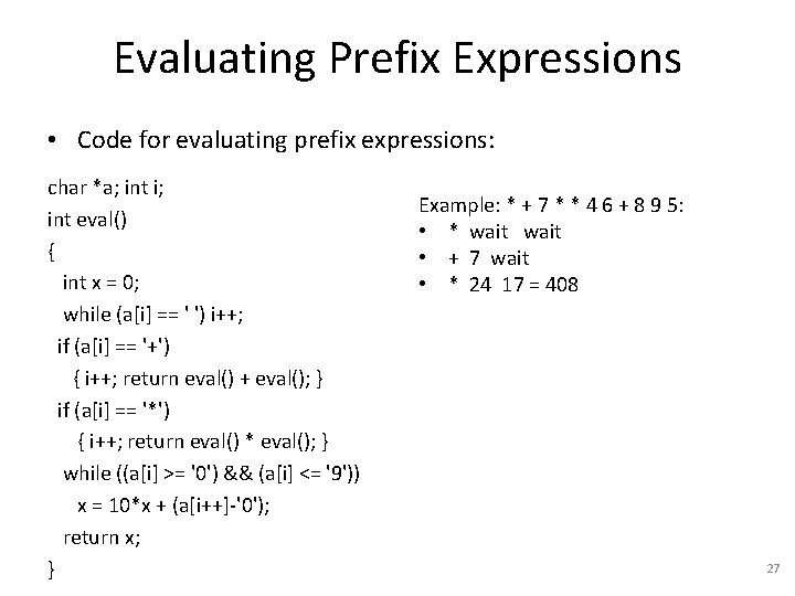
Evaluating Prefix Expressions • Code for evaluating prefix expressions: char *a; int i; int eval() { int x = 0; while (a[i] == ' ') i++; if (a[i] == '+') { i++; return eval() + eval(); } if (a[i] == '*') { i++; return eval() * eval(); } while ((a[i] >= '0') && (a[i] <= '9')) x = 10*x + (a[i++]-'0'); return x; } Example: * + 7 * * 4 6 + 8 9 5: • * wait • + 7 wait • * 24 17 = 408 27

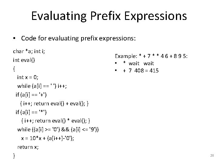
Evaluating Prefix Expressions • Code for evaluating prefix expressions: char *a; int i; int eval() { int x = 0; while (a[i] == ' ') i++; if (a[i] == '+') { i++; return eval() + eval(); } if (a[i] == '*') { i++; return eval() * eval(); } while ((a[i] >= '0') && (a[i] <= '9')) x = 10*x + (a[i++]-'0'); return x; } Example: * + 7 * * 4 6 + 8 9 5: • * wait • + 7 408 = 415 28

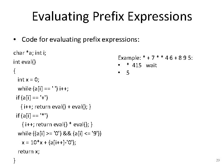
Evaluating Prefix Expressions • Code for evaluating prefix expressions: char *a; int i; int eval() { int x = 0; while (a[i] == ' ') i++; if (a[i] == '+') { i++; return eval() + eval(); } if (a[i] == '*') { i++; return eval() * eval(); } while ((a[i] >= '0') && (a[i] <= '9')) x = 10*x + (a[i++]-'0'); return x; } Example: * + 7 * * 4 6 + 8 9 5: • * 415 wait • 5 29

Evaluating Prefix Expressions • Code for evaluating prefix expressions: char *a; int i; int eval() { int x = 0; while (a[i] == ' ') i++; if (a[i] == '+') { i++; return eval() + eval(); } if (a[i] == '*') { i++; return eval() * eval(); } while ((a[i] >= '0') && (a[i] <= '9')) x = 10*x + (a[i++]-'0'); return x; } Example: * + 7 * * 4 6 + 8 9 5: • * 415 5 = 2075 30

Recursive Vs. Non-Recursive Implementations • In some cases, recursive functions are much easier to read. • They make crystal clear the mathematical structure of the algorithm. • To process recursive data types, such as nodes, oftentimes it is easy to write recursive functions. • Example: int count(link x) – count how many links there are between x and the end of the list. – Recursive solution? – Base case? Recursive function? 31

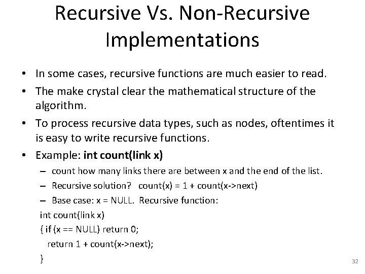
Recursive Vs. Non-Recursive Implementations • In some cases, recursive functions are much easier to read. • The make crystal clear the mathematical structure of the algorithm. • To process recursive data types, such as nodes, oftentimes it is easy to write recursive functions. • Example: int count(link x) – count how many links there are between x and the end of the list. – Recursive solution? count(x) = 1 + count(x->next) – Base case: x = NULL. Recursive function: int count(link x) { if (x == NULL) return 0; return 1 + count(x->next); } 32

Recursive Vs. Non-Recursive Implementations • In some cases, recursive functions are much easier to read. – They make crystal clear the mathematical structure of the algorithm. • To process recursive data types, such as nodes, oftentimes it is easy to write recursive functions. • However, any recursive function can also be written in a nonrecursive way. • Oftentimes recursive functions run slower. Why? 33

Recursive Vs. Non-Recursive Implementations • In some cases, recursive functions are much easier to read. – They make crystal clear the mathematical structure of the algorithm. • To process recursive data types, such as nodes, oftentimes it is easy to write recursive functions. • However, any recursive function can also be written in a nonrecursive way. • Oftentimes recursive functions run slower. Why? – Recursive functions generate many function calls. – The CPU has to pay a price (perform a certain number of operations) for each function call. • Non-recursive implementations are oftentimes somewhat uglier (and more buggy, harder to debug) but more efficient. – Compromise: make first version recursive, second non-recursive. 34

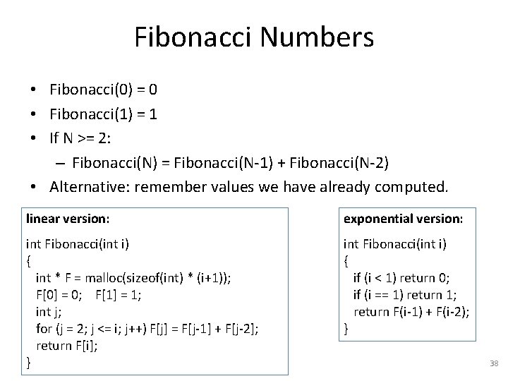
Fibonacci Numbers • Fibonacci(0) = 0 • Fibonacci(1) = 1 • If N >= 2: – Fibonacci(N) = Fibonacci(N-1) + Fibonacci(N-2) • How can we write a function that computes Fibonacci numbers? 35

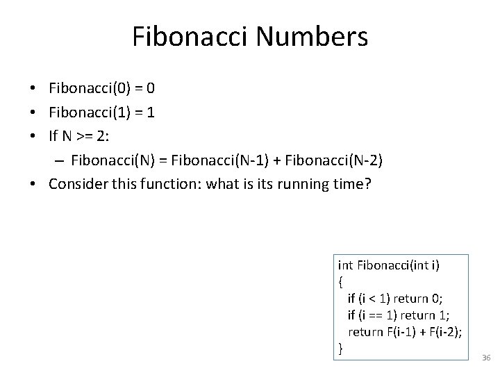
Fibonacci Numbers • Fibonacci(0) = 0 • Fibonacci(1) = 1 • If N >= 2: – Fibonacci(N) = Fibonacci(N-1) + Fibonacci(N-2) • Consider this function: what is its running time? int Fibonacci(int i) { if (i < 1) return 0; if (i == 1) return 1; return F(i-1) + F(i-2); } 36

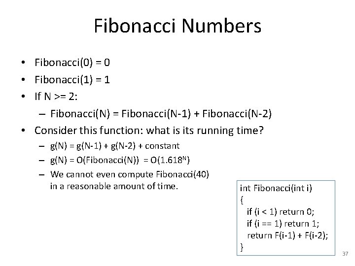
Fibonacci Numbers • Fibonacci(0) = 0 • Fibonacci(1) = 1 • If N >= 2: – Fibonacci(N) = Fibonacci(N-1) + Fibonacci(N-2) • Consider this function: what is its running time? – g(N) = g(N-1) + g(N-2) + constant – g(N) = O(Fibonacci(N)) = O(1. 618 N) – We cannot even compute Fibonacci(40) in a reasonable amount of time. int Fibonacci(int i) { if (i < 1) return 0; if (i == 1) return 1; return F(i-1) + F(i-2); } 37

Fibonacci Numbers • Fibonacci(0) = 0 • Fibonacci(1) = 1 • If N >= 2: – Fibonacci(N) = Fibonacci(N-1) + Fibonacci(N-2) • Alternative: remember values we have already computed. linear version: exponential version: int Fibonacci(int i) { int * F = malloc(sizeof(int) * (i+1)); F[0] = 0; F[1] = 1; int j; for (j = 2; j <= i; j++) F[j] = F[j-1] + F[j-2]; return F[i]; } int Fibonacci(int i) { if (i < 1) return 0; if (i == 1) return 1; return F(i-1) + F(i-2); } 38

Bottom-up Dynamic Programming • The technique we have just used is called bottom-up dynamic programming. • It is widely applicable, in a large variety of problems. 39

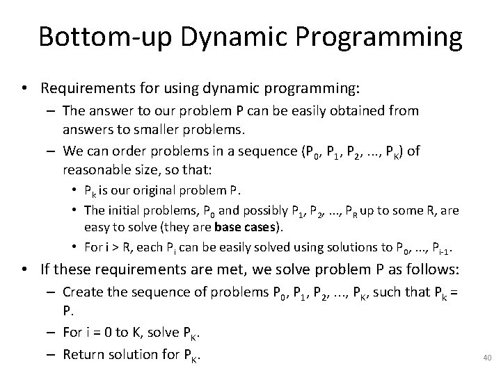
Bottom-up Dynamic Programming • Requirements for using dynamic programming: – The answer to our problem P can be easily obtained from answers to smaller problems. – We can order problems in a sequence (P 0, P 1, P 2, . . . , PK) of reasonable size, so that: • Pk is our original problem P. • The initial problems, P 0 and possibly P 1, P 2, . . . , PR up to some R, are easy to solve (they are base cases). • For i > R, each Pi can be easily solved using solutions to P 0, . . . , Pi-1. • If these requirements are met, we solve problem P as follows: – Create the sequence of problems P 0, P 1, P 2, . . . , PK, such that Pk = P. – For i = 0 to K, solve PK. – Return solution for PK. 40

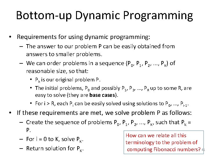
Bottom-up Dynamic Programming • Requirements for using dynamic programming: – The answer to our problem P can be easily obtained from answers to smaller problems. – We can order problems in a sequence (P 0, P 1, P 2, . . . , PK) of reasonable size, so that: • Pk is our original problem P. • The initial problems, P 0 and possibly P 1, P 2, . . . , PR up to some R, are easy to solve (they are base cases). • For i > R, each Pi can be easily solved using solutions to P 0, . . . , Pi-1. • If these requirements are met, we solve problem P as follows: – Create the sequence of problems P 0, P 1, P 2, . . . , PK, such that Pk = P. How can we relate all this – For i = 0 to K, solve PK. terminology to the problem of – Return solution for PK. computing Fibonacci numbers? 41

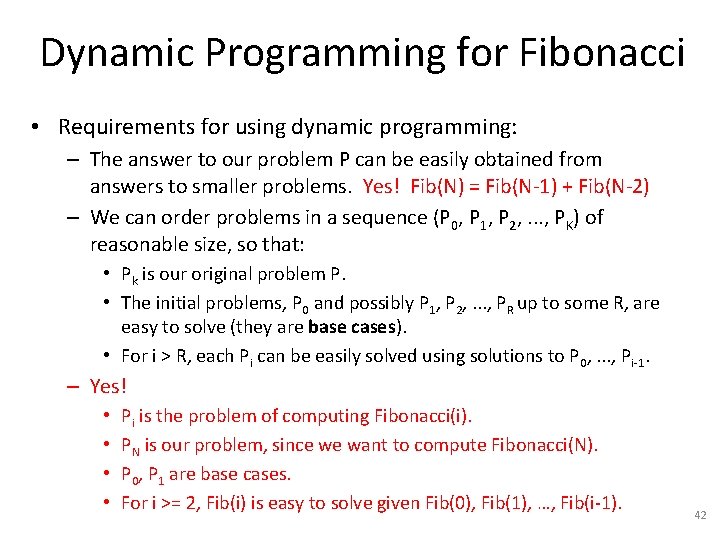
Dynamic Programming for Fibonacci • Requirements for using dynamic programming: – The answer to our problem P can be easily obtained from answers to smaller problems. Yes! Fib(N) = Fib(N-1) + Fib(N-2) – We can order problems in a sequence (P 0, P 1, P 2, . . . , PK) of reasonable size, so that: • Pk is our original problem P. • The initial problems, P 0 and possibly P 1, P 2, . . . , PR up to some R, are easy to solve (they are base cases). • For i > R, each Pi can be easily solved using solutions to P 0, . . . , Pi-1. – Yes! • • Pi is the problem of computing Fibonacci(i). PN is our problem, since we want to compute Fibonacci(N). P 0, P 1 are base cases. For i >= 2, Fib(i) is easy to solve given Fib(0), Fib(1), …, Fib(i-1). 42

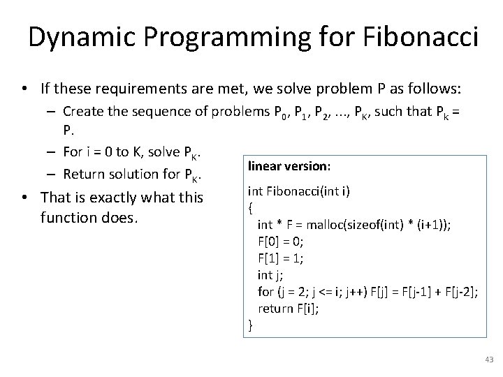
Dynamic Programming for Fibonacci • If these requirements are met, we solve problem P as follows: – Create the sequence of problems P 0, P 1, P 2, . . . , PK, such that Pk = P. – For i = 0 to K, solve PK. linear version: – Return solution for PK. • That is exactly what this function does. int Fibonacci(int i) { int * F = malloc(sizeof(int) * (i+1)); F[0] = 0; F[1] = 1; int j; for (j = 2; j <= i; j++) F[j] = F[j-1] + F[j-2]; return F[i]; } 43

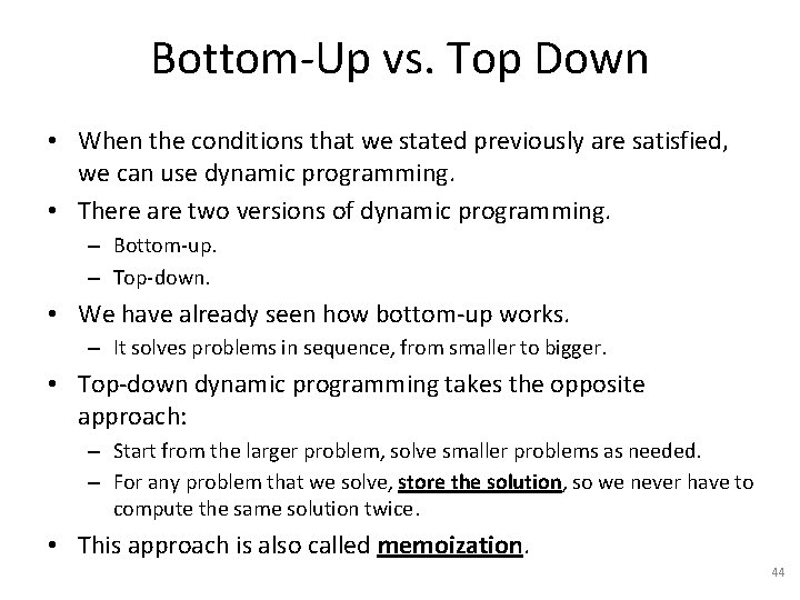
Bottom-Up vs. Top Down • When the conditions that we stated previously are satisfied, we can use dynamic programming. • There are two versions of dynamic programming. – Bottom-up. – Top-down. • We have already seen how bottom-up works. – It solves problems in sequence, from smaller to bigger. • Top-down dynamic programming takes the opposite approach: – Start from the larger problem, solve smaller problems as needed. – For any problem that we solve, store the solution, so we never have to compute the same solution twice. • This approach is also called memoization. 44

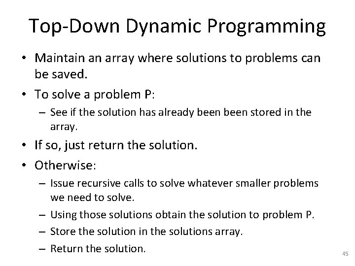
Top-Down Dynamic Programming • Maintain an array where solutions to problems can be saved. • To solve a problem P: – See if the solution has already been stored in the array. • If so, just return the solution. • Otherwise: – Issue recursive calls to solve whatever smaller problems we need to solve. – Using those solutions obtain the solution to problem P. – Store the solution in the solutions array. – Return the solution. 45

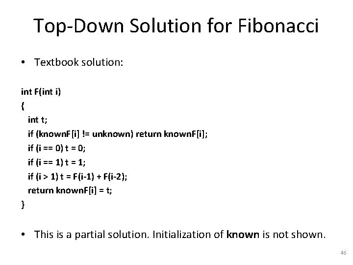
Top-Down Solution for Fibonacci • Textbook solution: int F(int i) { int t; if (known. F[i] != unknown) return known. F[i]; if (i == 0) t = 0; if (i == 1) t = 1; if (i > 1) t = F(i-1) + F(i-2); return known. F[i] = t; } • This is a partial solution. Initialization of known is not shown. 46

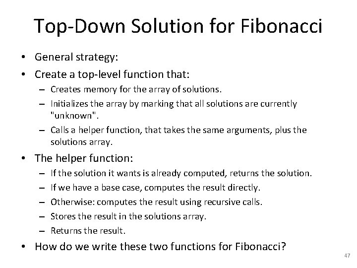
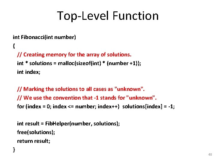
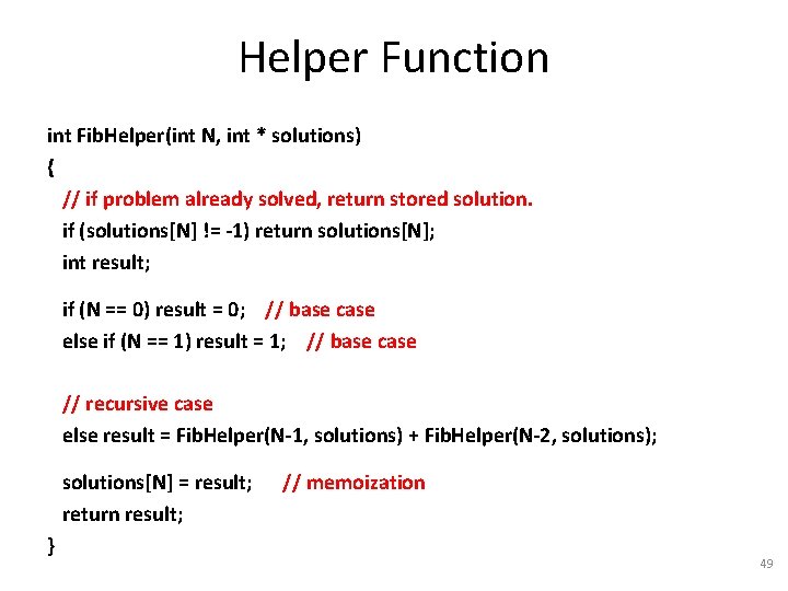
Top-Down Solution for Fibonacci • General strategy: • Create a top-level function that: – Creates memory for the array of solutions. – Initializes the array by marking that all solutions are currently "unknown". – Calls a helper function, that takes the same arguments, plus the solutions array. • The helper function: – – – If the solution it wants is already computed, returns the solution. If we have a base case, computes the result directly. Otherwise: computes the result using recursive calls. Stores the result in the solutions array. Returns the result. • How do we write these two functions for Fibonacci? 47

Top-Level Function int Fibonacci(int number) { // Creating memory for the array of solutions. int * solutions = malloc(sizeof(int) * (number +1)); int index; // Marking the solutions to all cases as "unknown". // We use the convention that -1 stands for "unknown". for (index = 0; index <= number; index++) solutions[index] = -1; int result = Fib. Helper(number, solutions); free(solutions); return result; } 48

Helper Function int Fib. Helper(int N, int * solutions) { // if problem already solved, return stored solution. if (solutions[N] != -1) return solutions[N]; int result; if (N == 0) result = 0; // base case else if (N == 1) result = 1; // base case // recursive case else result = Fib. Helper(N-1, solutions) + Fib. Helper(N-2, solutions); solutions[N] = result; return result; } // memoization 49

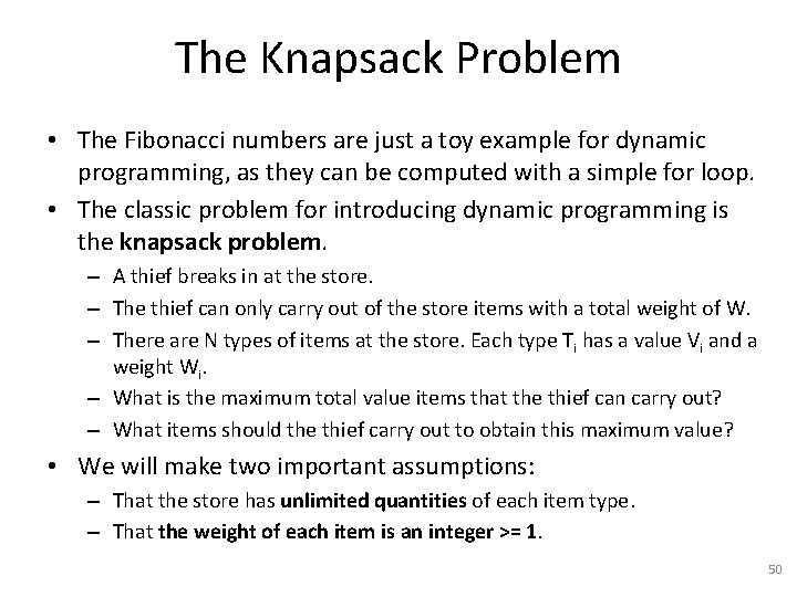
The Knapsack Problem • The Fibonacci numbers are just a toy example for dynamic programming, as they can be computed with a simple for loop. • The classic problem for introducing dynamic programming is the knapsack problem. – A thief breaks in at the store. – The thief can only carry out of the store items with a total weight of W. – There are N types of items at the store. Each type Ti has a value Vi and a weight Wi. – What is the maximum total value items that the thief can carry out? – What items should the thief carry out to obtain this maximum value? • We will make two important assumptions: – That the store has unlimited quantities of each item type. – That the weight of each item is an integer >= 1. 50

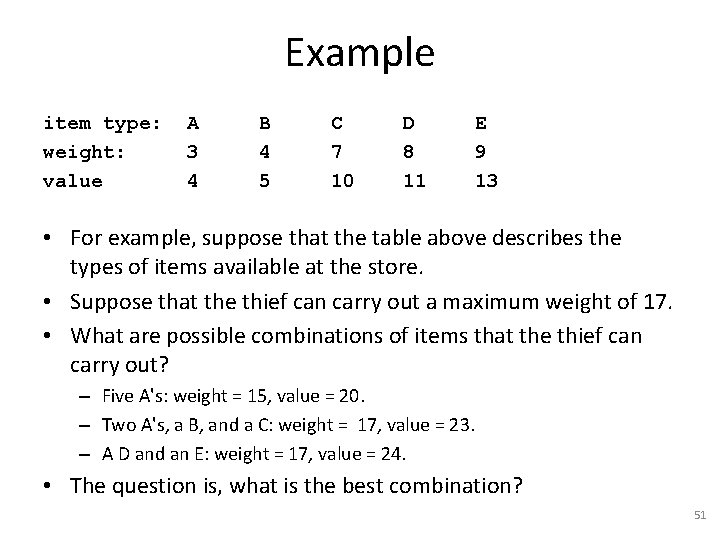
Example item type: weight: value A 3 4 B 4 5 C 7 10 D 8 11 E 9 13 • For example, suppose that the table above describes the types of items available at the store. • Suppose that the thief can carry out a maximum weight of 17. • What are possible combinations of items that the thief can carry out? – Five A's: weight = 15, value = 20. – Two A's, a B, and a C: weight = 17, value = 23. – A D and an E: weight = 17, value = 24. • The question is, what is the best combination? 51

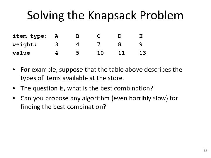
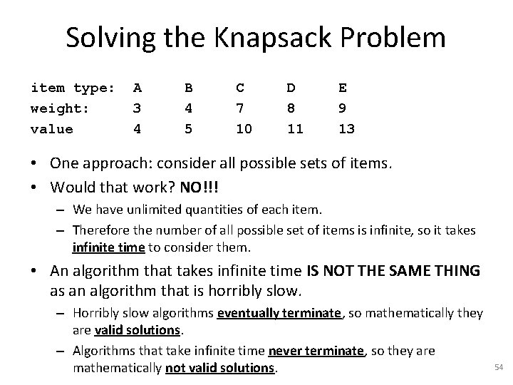
Solving the Knapsack Problem item type: weight: value A 3 4 B 4 5 C 7 10 D 8 11 E 9 13 • For example, suppose that the table above describes the types of items available at the store. • The question is, what is the best combination? • Can you propose any algorithm (even horribly slow) for finding the best combination? 52

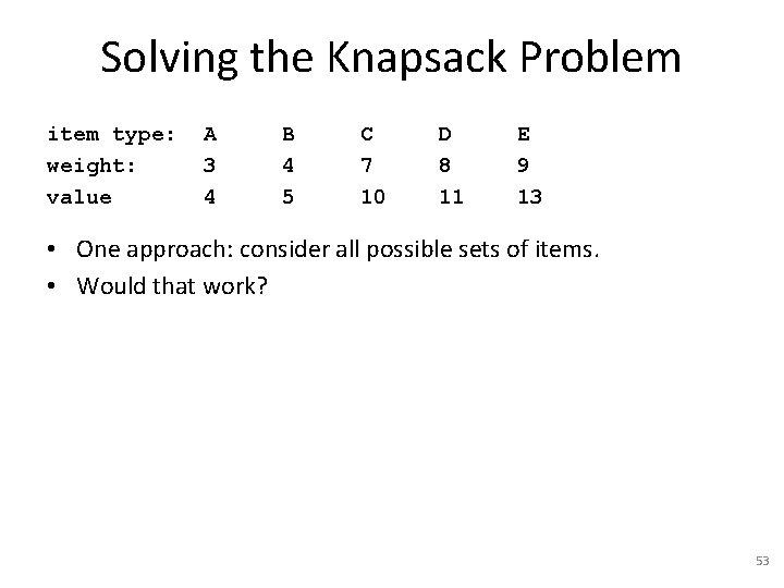
Solving the Knapsack Problem item type: weight: value A 3 4 B 4 5 C 7 10 D 8 11 E 9 13 • One approach: consider all possible sets of items. • Would that work? 53

Solving the Knapsack Problem item type: weight: value A 3 4 B 4 5 C 7 10 D 8 11 E 9 13 • One approach: consider all possible sets of items. • Would that work? NO!!! – We have unlimited quantities of each item. – Therefore the number of all possible set of items is infinite, so it takes infinite time to consider them. • An algorithm that takes infinite time IS NOT THE SAME THING as an algorithm that is horribly slow. – Horribly slow algorithms eventually terminate, so mathematically they are valid solutions. – Algorithms that take infinite time never terminate, so they are mathematically not valid solutions. 54

Solving the Knapsack Problem • To use dynamic programming, we need to identify whether solving our problem can be done easily if we have already sold smaller problems. • What would be a smaller problem? – Our original problem is: find the set of items with weight <= W that has the most value. 55

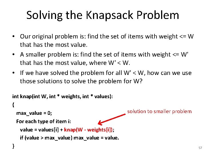
Solving the Knapsack Problem • To use dynamic programming, we need to identify whether solving our problem can be done easily if we have already sold smaller problems. • What would be a smaller problem? – Our original problem is: find the set of items with weight <= W that has the most value. • A smaller problem is: find the set of items with weight <= W' that has the most value, where W' < W. • If we have solved the problem for all W' < W, how can we use those solutions to solve the problem for W? 56

Solving the Knapsack Problem • Our original problem is: find the set of items with weight <= W that has the most value. • A smaller problem is: find the set of items with weight <= W' that has the most value, where W' < W. • If we have solved the problem for all W' < W, how can we use those solutions to solve the problem for W? int knap(int W, int * weights, int * values): { max_value = 0; For each type of item i: value = values[i] + knap(W - weights[i]); if (value > max_value) max_value = value. } solution to smaller problem 57

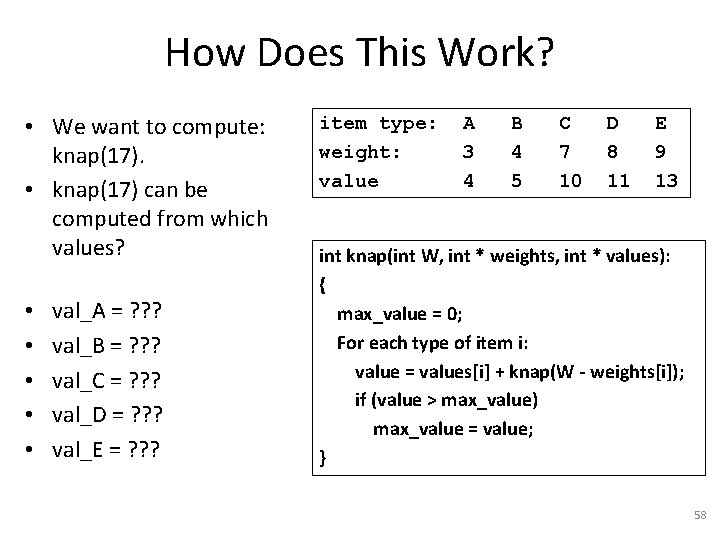
How Does This Work? • We want to compute: knap(17). • knap(17) can be computed from which values? • • • val_A = ? ? ? val_B = ? ? ? val_C = ? ? ? val_D = ? ? ? val_E = ? ? ? item type: weight: value A 3 4 B 4 5 C 7 10 D 8 11 E 9 13 int knap(int W, int * weights, int * values): { max_value = 0; For each type of item i: value = values[i] + knap(W - weights[i]); if (value > max_value) max_value = value; } 58

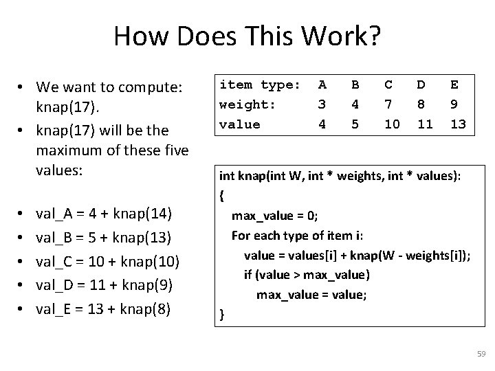
How Does This Work? • We want to compute: knap(17). • knap(17) will be the maximum of these five values: • • • val_A = 4 + knap(14) val_B = 5 + knap(13) val_C = 10 + knap(10) val_D = 11 + knap(9) val_E = 13 + knap(8) item type: weight: value A 3 4 B 4 5 C 7 10 D 8 11 E 9 13 int knap(int W, int * weights, int * values): { max_value = 0; For each type of item i: value = values[i] + knap(W - weights[i]); if (value > max_value) max_value = value; } 59

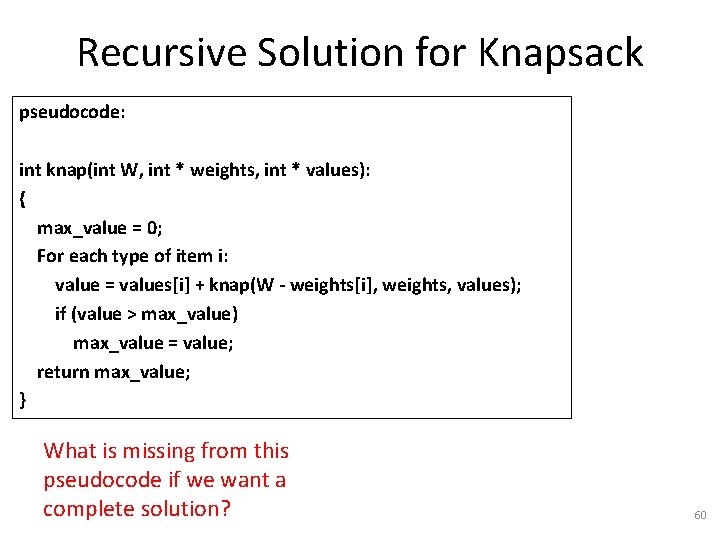
Recursive Solution for Knapsack pseudocode: int knap(int W, int * weights, int * values): { max_value = 0; For each type of item i: value = values[i] + knap(W - weights[i], weights, values); if (value > max_value) max_value = value; return max_value; } What is missing from this pseudocode if we want a complete solution? 60

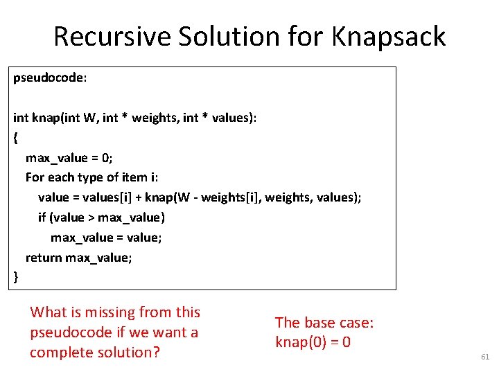
Recursive Solution for Knapsack pseudocode: int knap(int W, int * weights, int * values): { max_value = 0; For each type of item i: value = values[i] + knap(W - weights[i], weights, values); if (value > max_value) max_value = value; return max_value; } What is missing from this pseudocode if we want a complete solution? The base case: knap(0) = 0 61

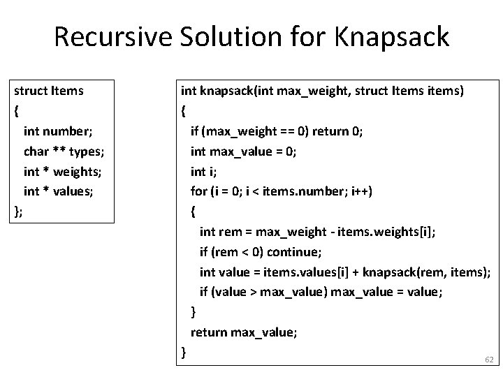
Recursive Solution for Knapsack struct Items { int number; char ** types; int * weights; int * values; }; int knapsack(int max_weight, struct Items items) { if (max_weight == 0) return 0; int max_value = 0; int i; for (i = 0; i < items. number; i++) { int rem = max_weight - items. weights[i]; if (rem < 0) continue; int value = items. values[i] + knapsack(rem, items); if (value > max_value) max_value = value; } return max_value; } 62

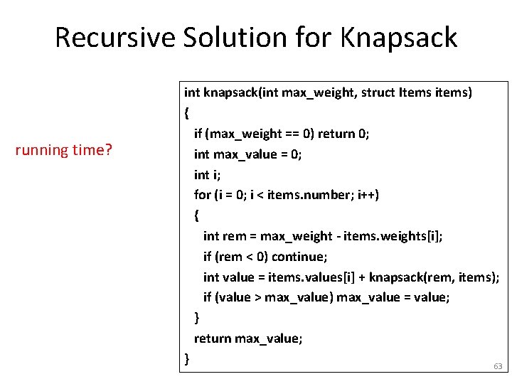
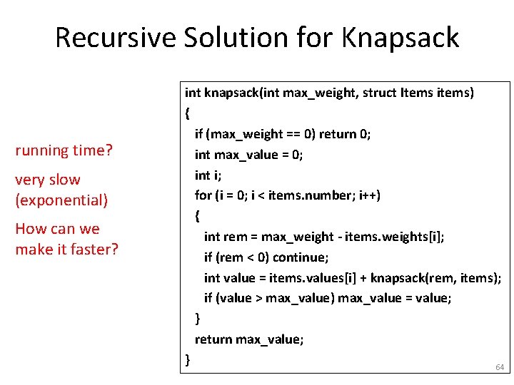
Recursive Solution for Knapsack running time? int knapsack(int max_weight, struct Items items) { if (max_weight == 0) return 0; int max_value = 0; int i; for (i = 0; i < items. number; i++) { int rem = max_weight - items. weights[i]; if (rem < 0) continue; int value = items. values[i] + knapsack(rem, items); if (value > max_value) max_value = value; } return max_value; } 63

Recursive Solution for Knapsack running time? very slow (exponential) How can we make it faster? int knapsack(int max_weight, struct Items items) { if (max_weight == 0) return 0; int max_value = 0; int i; for (i = 0; i < items. number; i++) { int rem = max_weight - items. weights[i]; if (rem < 0) continue; int value = items. values[i] + knapsack(rem, items); if (value > max_value) max_value = value; } return max_value; } 64

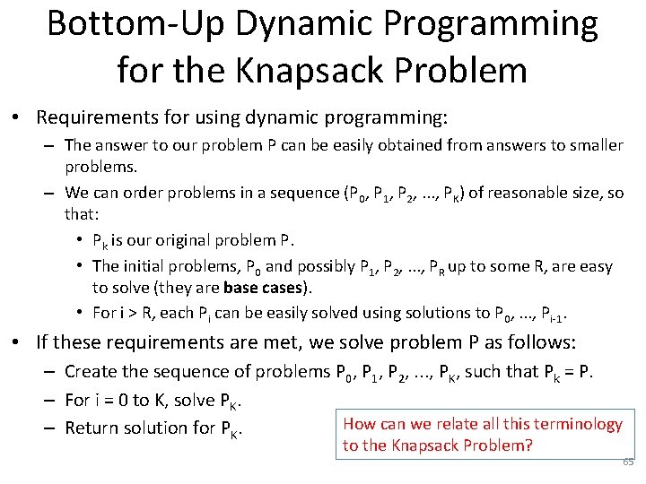
Bottom-Up Dynamic Programming for the Knapsack Problem • Requirements for using dynamic programming: – The answer to our problem P can be easily obtained from answers to smaller problems. – We can order problems in a sequence (P 0, P 1, P 2, . . . , PK) of reasonable size, so that: • Pk is our original problem P. • The initial problems, P 0 and possibly P 1, P 2, . . . , PR up to some R, are easy to solve (they are base cases). • For i > R, each Pi can be easily solved using solutions to P 0, . . . , Pi-1. • If these requirements are met, we solve problem P as follows: – Create the sequence of problems P 0, P 1, P 2, . . . , PK, such that Pk = P. – For i = 0 to K, solve PK. How can we relate all this terminology – Return solution for PK. to the Knapsack Problem? 65

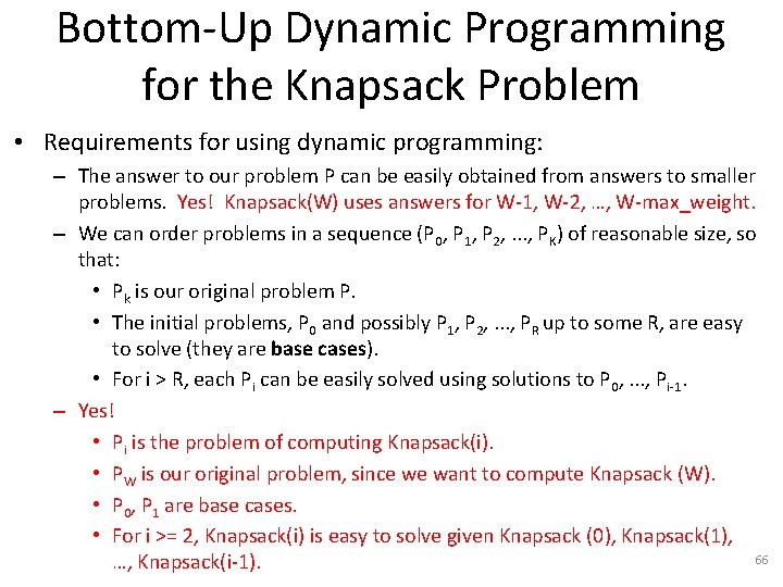
Bottom-Up Dynamic Programming for the Knapsack Problem • Requirements for using dynamic programming: – The answer to our problem P can be easily obtained from answers to smaller problems. Yes! Knapsack(W) uses answers for W-1, W-2, …, W-max_weight. – We can order problems in a sequence (P 0, P 1, P 2, . . . , PK) of reasonable size, so that: • Pk is our original problem P. • The initial problems, P 0 and possibly P 1, P 2, . . . , PR up to some R, are easy to solve (they are base cases). • For i > R, each Pi can be easily solved using solutions to P 0, . . . , Pi-1. – Yes! • Pi is the problem of computing Knapsack(i). • PW is our original problem, since we want to compute Knapsack (W). • P 0, P 1 are base cases. • For i >= 2, Knapsack(i) is easy to solve given Knapsack (0), Knapsack(1), 66 …, Knapsack(i-1).

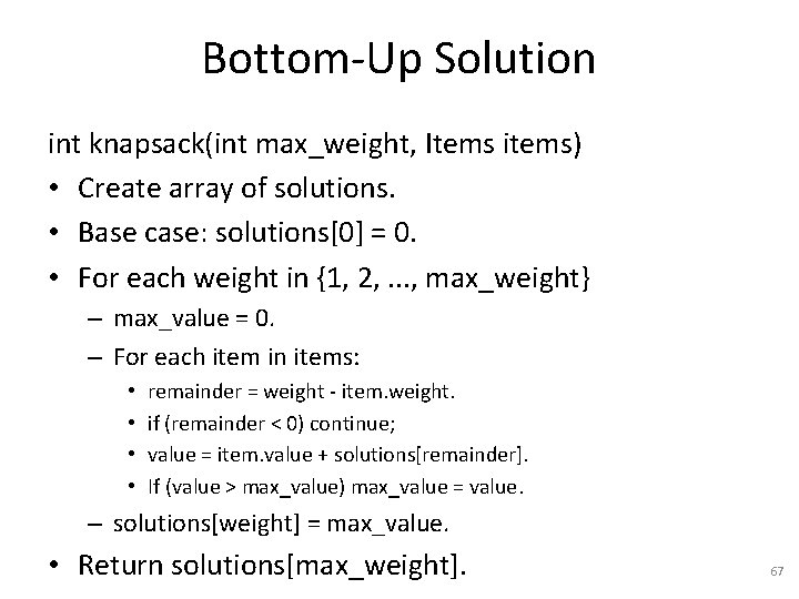
Bottom-Up Solution int knapsack(int max_weight, Items items) • Create array of solutions. • Base case: solutions[0] = 0. • For each weight in {1, 2, . . . , max_weight} – max_value = 0. – For each item in items: • • remainder = weight - item. weight. if (remainder < 0) continue; value = item. value + solutions[remainder]. If (value > max_value) max_value = value. – solutions[weight] = max_value. • Return solutions[max_weight]. 67

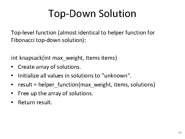
Top-Down Solution Top-level function (almost identical to helper function for Fibonacci top-down solution): int knapsack(int max_weight, Items items) • Create array of solutions. • Initialize all values in solutions to "unknown". • result = helper_function(max_weight, items, solutions) • Free up the array of solutions. • Return result. 68

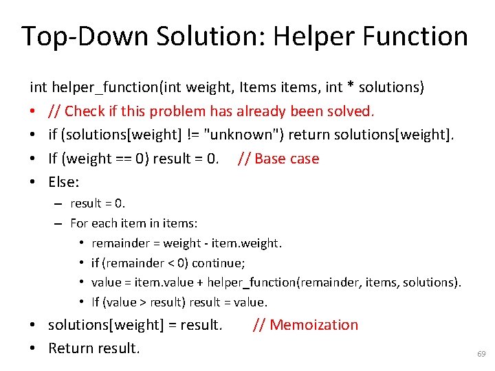
Top-Down Solution: Helper Function int helper_function(int weight, Items items, int * solutions) • // Check if this problem has already been solved. • if (solutions[weight] != "unknown") return solutions[weight]. • If (weight == 0) result = 0. // Base case • Else: – result = 0. – For each item in items: • remainder = weight - item. weight. • if (remainder < 0) continue; • value = item. value + helper_function(remainder, items, solutions). • If (value > result) result = value. • solutions[weight] = result. • Return result. // Memoization 69

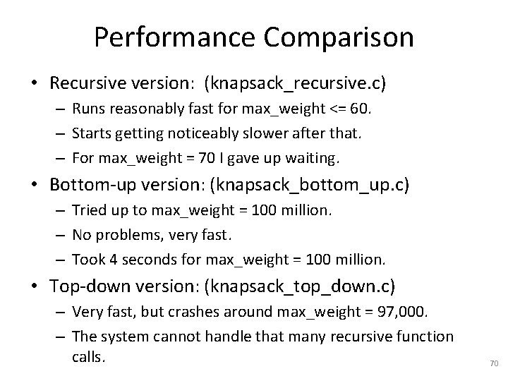
Performance Comparison • Recursive version: (knapsack_recursive. c) – Runs reasonably fast for max_weight <= 60. – Starts getting noticeably slower after that. – For max_weight = 70 I gave up waiting. • Bottom-up version: (knapsack_bottom_up. c) – Tried up to max_weight = 100 million. – No problems, very fast. – Took 4 seconds for max_weight = 100 million. • Top-down version: (knapsack_top_down. c) – Very fast, but crashes around max_weight = 97, 000. – The system cannot handle that many recursive function calls. 70

Limitation of All Three Solutions • Each of the solutions returns a number. • Is a single number all we want to answer our original problem? 71

Limitation of All Three Solutions • Each of the solutions returns a number. • Is a single number all we want to answer our original problem? – No. Our original problem was to find the best set of items. – It is nice to know the best possible value we can achieve. – But, we also want to know the actual set of items that achieves that value. • This will be left as a homework for you. 72

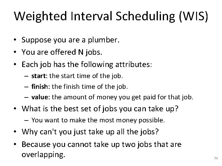
Weighted Interval Scheduling (WIS) • Suppose you are a plumber. • You are offered N jobs. • Each job has the following attributes: – start: the start time of the job. – finish: the finish time of the job. – value: the amount of money you get paid for that job. • What is the best set of jobs you can take up? – You want to make the most money possible. • Why can't you just take up all the jobs? 73

Weighted Interval Scheduling (WIS) • Suppose you are a plumber. • You are offered N jobs. • Each job has the following attributes: – start: the start time of the job. – finish: the finish time of the job. – value: the amount of money you get paid for that job. • What is the best set of jobs you can take up? – You want to make the most money possible. • Why can't you just take up all the jobs? • Because you cannot take up two jobs that are overlapping. 74

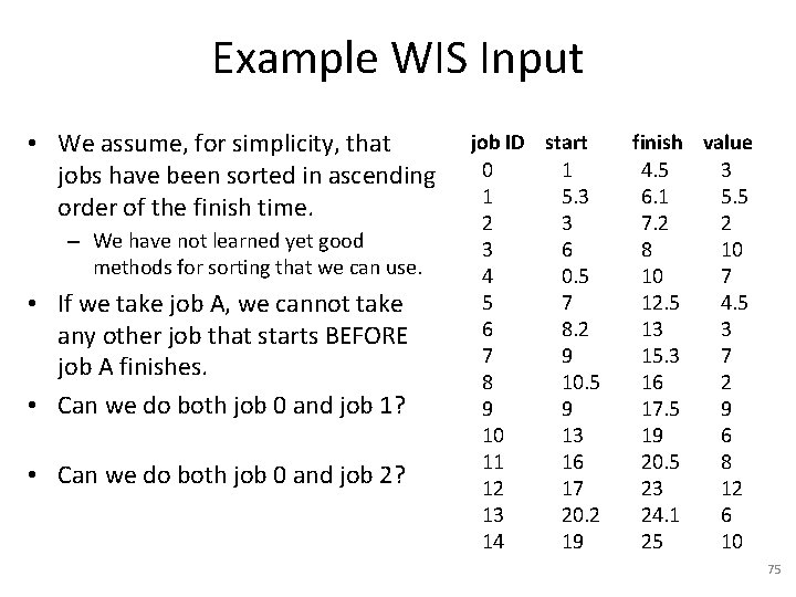
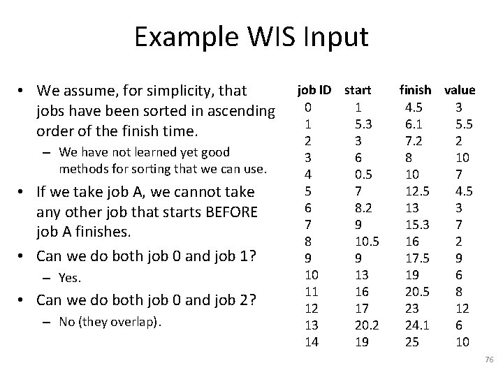
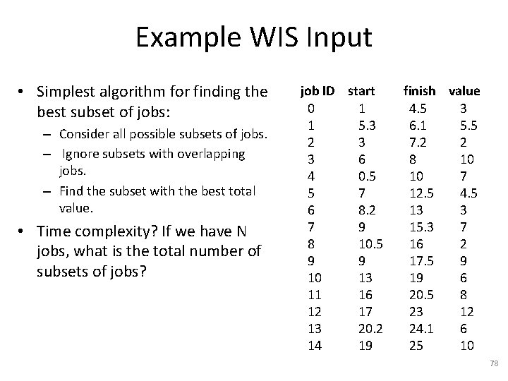
Example WIS Input • We assume, for simplicity, that jobs have been sorted in ascending order of the finish time. – We have not learned yet good methods for sorting that we can use. • If we take job A, we cannot take any other job that starts BEFORE job A finishes. • Can we do both job 0 and job 1? • Can we do both job 0 and job 2? job ID start 0 1 1 5. 3 2 3 3 6 4 0. 5 5 7 6 8. 2 7 9 8 10. 5 9 9 10 13 11 16 12 17 13 20. 2 14 19 finish value 4. 5 3 6. 1 5. 5 7. 2 2 8 10 10 7 12. 5 4. 5 13 3 15. 3 7 16 2 17. 5 9 19 6 20. 5 8 23 12 24. 1 6 25 10 75

Example WIS Input • We assume, for simplicity, that jobs have been sorted in ascending order of the finish time. – We have not learned yet good methods for sorting that we can use. • If we take job A, we cannot take any other job that starts BEFORE job A finishes. • Can we do both job 0 and job 1? – Yes. • Can we do both job 0 and job 2? – No (they overlap). job ID start 0 1 1 5. 3 2 3 3 6 4 0. 5 5 7 6 8. 2 7 9 8 10. 5 9 9 10 13 11 16 12 17 13 20. 2 14 19 finish value 4. 5 3 6. 1 5. 5 7. 2 2 8 10 10 7 12. 5 4. 5 13 3 15. 3 7 16 2 17. 5 9 19 6 20. 5 8 23 12 24. 1 6 25 10 76

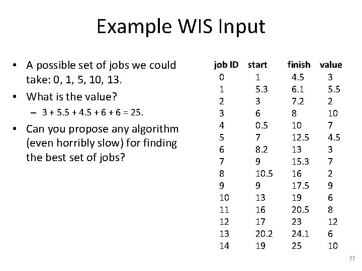
Example WIS Input • A possible set of jobs we could take: 0, 1, 5, 10, 13. • What is the value? – 3 + 5. 5 + 4. 5 + 6 = 25. • Can you propose any algorithm (even horribly slow) for finding the best set of jobs? job ID start 0 1 1 5. 3 2 3 3 6 4 0. 5 5 7 6 8. 2 7 9 8 10. 5 9 9 10 13 11 16 12 17 13 20. 2 14 19 finish value 4. 5 3 6. 1 5. 5 7. 2 2 8 10 10 7 12. 5 4. 5 13 3 15. 3 7 16 2 17. 5 9 19 6 20. 5 8 23 12 24. 1 6 25 10 77

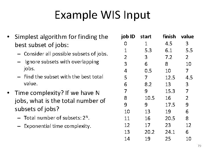
Example WIS Input • Simplest algorithm for finding the best subset of jobs: – Consider all possible subsets of jobs. – Ignore subsets with overlapping jobs. – Find the subset with the best total value. • Time complexity? If we have N jobs, what is the total number of subsets of jobs? job ID start 0 1 1 5. 3 2 3 3 6 4 0. 5 5 7 6 8. 2 7 9 8 10. 5 9 9 10 13 11 16 12 17 13 20. 2 14 19 finish value 4. 5 3 6. 1 5. 5 7. 2 2 8 10 10 7 12. 5 4. 5 13 3 15. 3 7 16 2 17. 5 9 19 6 20. 5 8 23 12 24. 1 6 25 10 78

Example WIS Input • Simplest algorithm for finding the best subset of jobs: – Consider all possible subsets of jobs. – Ignore subsets with overlapping jobs. – Find the subset with the best total value. • Time complexity? If we have N jobs, what is the total number of subsets of jobs? – Total number of subsets: 2 N. – Exponential time complexity. job ID start 0 1 1 5. 3 2 3 3 6 4 0. 5 5 7 6 8. 2 7 9 8 10. 5 9 9 10 13 11 16 12 17 13 20. 2 14 19 finish value 4. 5 3 6. 1 5. 5 7. 2 2 8 10 10 7 12. 5 4. 5 13 3 15. 3 7 16 2 17. 5 9 19 6 20. 5 8 23 12 24. 1 6 25 10 79

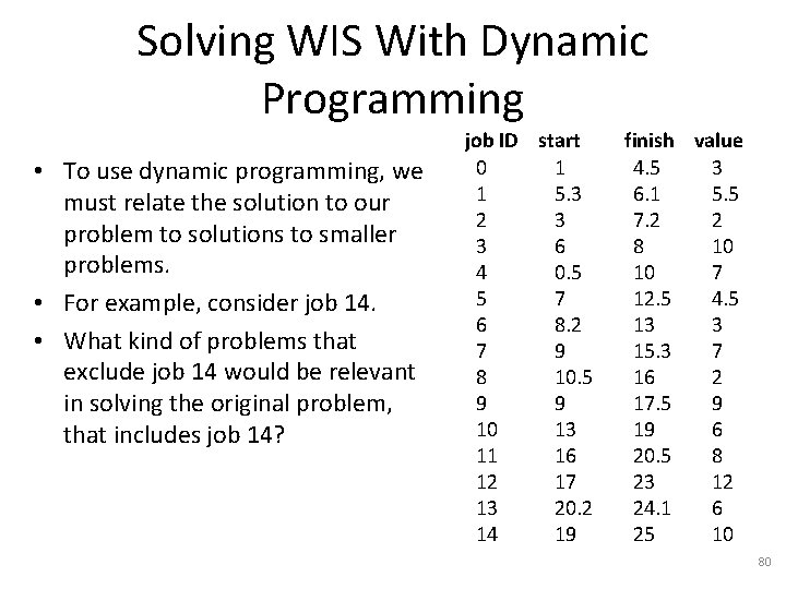
Solving WIS With Dynamic Programming • To use dynamic programming, we must relate the solution to our problem to solutions to smaller problems. • For example, consider job 14. • What kind of problems that exclude job 14 would be relevant in solving the original problem, that includes job 14? job ID start 0 1 1 5. 3 2 3 3 6 4 0. 5 5 7 6 8. 2 7 9 8 10. 5 9 9 10 13 11 16 12 17 13 20. 2 14 19 finish value 4. 5 3 6. 1 5. 5 7. 2 2 8 10 10 7 12. 5 4. 5 13 3 15. 3 7 16 2 17. 5 9 19 6 20. 5 8 23 12 24. 1 6 25 10 80

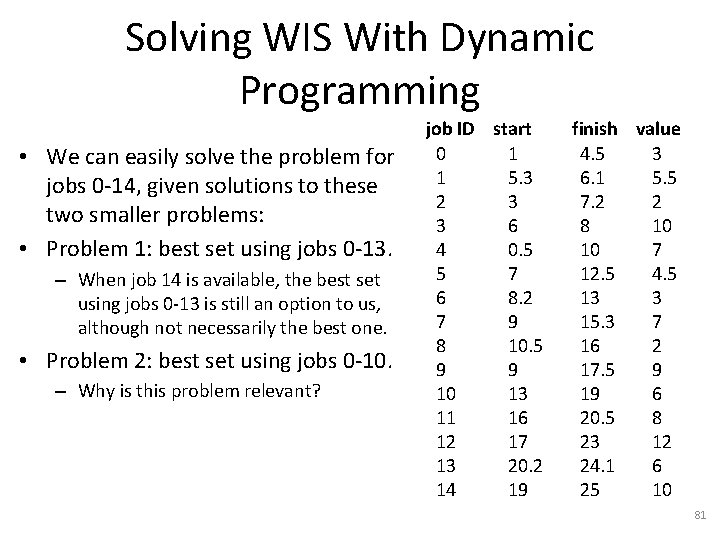
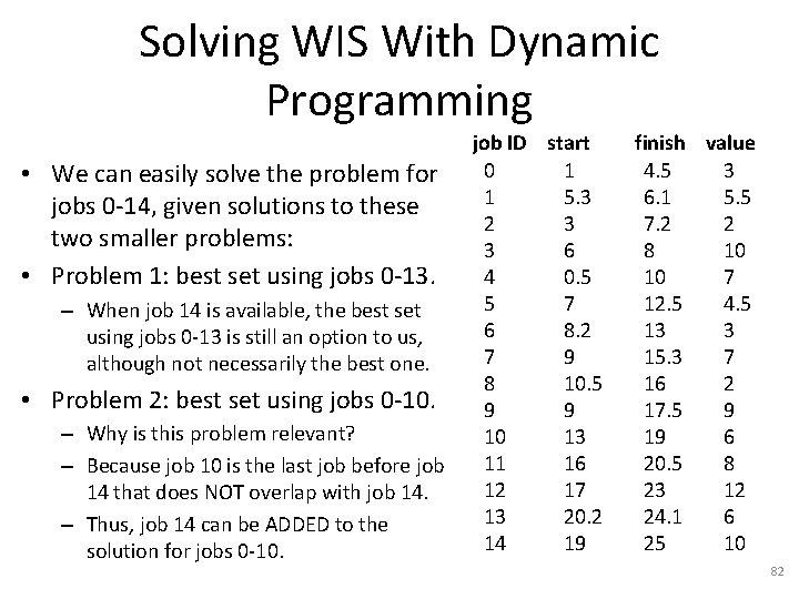
Solving WIS With Dynamic Programming • We can easily solve the problem for jobs 0 -14, given solutions to these two smaller problems: • Problem 1: best set using jobs 0 -13. – When job 14 is available, the best set using jobs 0 -13 is still an option to us, although not necessarily the best one. • Problem 2: best set using jobs 0 -10. – Why is this problem relevant? job ID start 0 1 1 5. 3 2 3 3 6 4 0. 5 5 7 6 8. 2 7 9 8 10. 5 9 9 10 13 11 16 12 17 13 20. 2 14 19 finish value 4. 5 3 6. 1 5. 5 7. 2 2 8 10 10 7 12. 5 4. 5 13 3 15. 3 7 16 2 17. 5 9 19 6 20. 5 8 23 12 24. 1 6 25 10 81

Solving WIS With Dynamic Programming • We can easily solve the problem for jobs 0 -14, given solutions to these two smaller problems: • Problem 1: best set using jobs 0 -13. – When job 14 is available, the best set using jobs 0 -13 is still an option to us, although not necessarily the best one. • Problem 2: best set using jobs 0 -10. – Why is this problem relevant? – Because job 10 is the last job before job 14 that does NOT overlap with job 14. – Thus, job 14 can be ADDED to the solution for jobs 0 -10. job ID start 0 1 1 5. 3 2 3 3 6 4 0. 5 5 7 6 8. 2 7 9 8 10. 5 9 9 10 13 11 16 12 17 13 20. 2 14 19 finish value 4. 5 3 6. 1 5. 5 7. 2 2 8 10 10 7 12. 5 4. 5 13 3 15. 3 7 16 2 17. 5 9 19 6 20. 5 8 23 12 24. 1 6 25 10 82

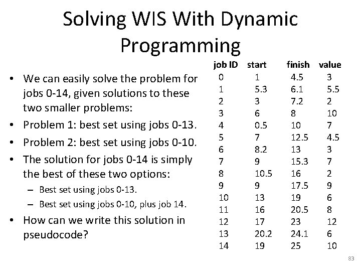
Solving WIS With Dynamic Programming • We can easily solve the problem for jobs 0 -14, given solutions to these two smaller problems: • Problem 1: best set using jobs 0 -13. • Problem 2: best set using jobs 0 -10. • The solution for jobs 0 -14 is simply the best of these two options: – Best set using jobs 0 -13. – Best set using jobs 0 -10, plus job 14. • How can we write this solution in pseudocode? job ID start 0 1 1 5. 3 2 3 3 6 4 0. 5 5 7 6 8. 2 7 9 8 10. 5 9 9 10 13 11 16 12 17 13 20. 2 14 19 finish value 4. 5 3 6. 1 5. 5 7. 2 2 8 10 10 7 12. 5 4. 5 13 3 15. 3 7 16 2 17. 5 9 19 6 20. 5 8 23 12 24. 1 6 25 10 83

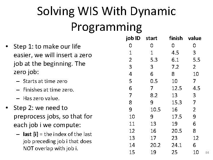
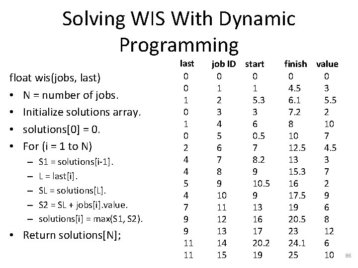
Solving WIS With Dynamic Programming • Step 1: to make our life easier, we will insert a zero job at the beginning. The zero job: – Starts at time zero – Finishes at time zero. – Has zero value. • Step 2: we need to preprocess jobs, so that for each job i we compute: – last [i] = the index of the last job preceding job i that does NOT overlap with job i. job ID start 0 0 1 1 2 5. 3 3 3 4 6 5 0. 5 6 7 7 8. 2 8 9 9 10. 5 10 9 11 13 12 16 13 17 14 20. 2 15 19 finish value 0 0 4. 5 3 6. 1 5. 5 7. 2 2 8 10 10 7 12. 5 4. 5 13 3 15. 3 7 16 2 17. 5 9 19 6 20. 5 8 23 12 24. 1 6 25 10 84

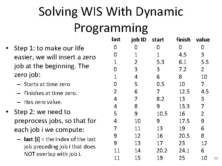
Solving WIS With Dynamic Programming • Step 1: to make our life easier, we will insert a zero job at the beginning. The zero job: – Starts at time zero – Finishes at time zero. – Has zero value. • Step 2: we need to preprocess jobs, so that for each job i we compute: – last [i] = the index of the last job preceding job i that does NOT overlap with job i. last 0 0 1 0 2 4 4 5 4 7 9 9 11 11 job ID start 0 0 1 1 2 5. 3 3 3 4 6 5 0. 5 6 7 7 8. 2 8 9 9 10. 5 10 9 11 13 12 16 13 17 14 20. 2 15 19 finish value 0 0 4. 5 3 6. 1 5. 5 7. 2 2 8 10 10 7 12. 5 4. 5 13 3 15. 3 7 16 2 17. 5 9 19 6 20. 5 8 23 12 24. 1 6 25 10 85

Solving WIS With Dynamic Programming float wis(jobs, last) • N = number of jobs. • Initialize solutions array. • solutions[0] = 0. • For (i = 1 to N) – – – S 1 = solutions[i-1]. L = last[i]. SL = solutions[L]. S 2 = SL + jobs[i]. value. solutions[i] = max(S 1, S 2). • Return solutions[N]; last 0 0 1 0 2 4 4 5 4 7 9 9 11 11 job ID start 0 0 1 1 2 5. 3 3 3 4 6 5 0. 5 6 7 7 8. 2 8 9 9 10. 5 10 9 11 13 12 16 13 17 14 20. 2 15 19 finish value 0 0 4. 5 3 6. 1 5. 5 7. 2 2 8 10 10 7 12. 5 4. 5 13 3 15. 3 7 16 2 17. 5 9 19 6 20. 5 8 23 12 24. 1 6 25 10 86

Backtracking • As in our solution to the knapsack problem, the pseudocode we just saw returns a number: – The best total value we can achieve. • In addition to the best value, we also want to know the set of jobs that achieves that value. • This is a general issue in dynamic programming. • How can we address it? 87

Backtracking • As in our solution to the knapsack problem, the pseudocode we just saw returns a number: – The best total value we can achieve. • In addition to the best value, we also want to know the set of jobs that achieves that value. • This is a general issue in dynamic programming. • There is a general solution, called backtracking. • The key idea is: – In DP the final solution is always built from smaller solutions. – At each smaller problem, we have to choose which (even smaller) solutions to use for solving that problem. – We must record, for each smaller problem, the choice we made. – At the end, we backtrack and recover the individual decisions that led to the best solution. 88

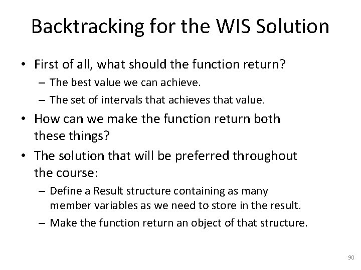
Backtracking for the WIS Solution • First of all, what should the function return? 89

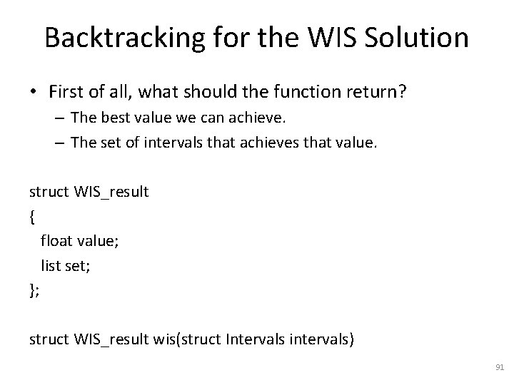
Backtracking for the WIS Solution • First of all, what should the function return? – The best value we can achieve. – The set of intervals that achieves that value. • How can we make the function return both these things? • The solution that will be preferred throughout the course: – Define a Result structure containing as many member variables as we need to store in the result. – Make the function return an object of that structure. 90

Backtracking for the WIS Solution • First of all, what should the function return? – The best value we can achieve. – The set of intervals that achieves that value. struct WIS_result { float value; list set; }; struct WIS_result wis(struct Intervals intervals) 91

Backtracking Solution Result wis(jobs, last) • N = number of jobs. • solutions[0] = 0. • For (i = 1 to N) – – – L = last[i]. SL = solutions[L]. S 1 = solutions[i-1]. S 2 = SL + jobs[i]. value. solutions[i] = max(S 1, S 2). • How can we keep track of the decisions we make? last 0 0 1 0 2 4 4 5 4 7 9 9 11 11 job ID start 0 0 1 1 2 5. 3 3 3 4 6 5 0. 5 6 7 7 8. 2 8 9 9 10. 5 10 9 11 13 12 16 13 17 14 20. 2 15 19 finish value 0 0 4. 5 3 6. 1 5. 5 7. 2 2 8 10 10 7 12. 5 4. 5 13 3 15. 3 7 16 2 17. 5 9 19 6 20. 5 8 23 12 24. 1 6 25 10 92

Backtracking Solution Result wis(jobs, last) • N = number of jobs. • solutions[0] = 0. • For (i = 1 to N) – – – L = last[i]. SL = solutions[L]. S 1 = solutions[i-1]. S 2 = SL + jobs[i]. value. solutions[i] = max(S 1, S 2). • How can we keep track of the decisions we make? • Remember the last job of each solution. last 0 0 1 0 2 4 4 5 4 7 9 9 11 11 job ID start 0 0 1 1 2 5. 3 3 3 4 6 5 0. 5 6 7 7 8. 2 8 9 9 10. 5 10 9 11 13 12 16 13 17 14 20. 2 15 19 finish value 0 0 4. 5 3 6. 1 5. 5 7. 2 2 8 10 10 7 12. 5 4. 5 13 3 15. 3 7 16 2 17. 5 9 19 6 20. 5 8 23 12 24. 1 6 25 10 93

Backtracking Solution Result wis(jobs, last) • N = number of jobs. • solutions[0] = 0. • used[0] = 0. • For (i = 1 to N) – – – – L = last[i]. SL = solutions[L]. S 1 = solutions[i-1]. S 2 = SL + jobs[i]. value. solutions[i] = max(S 1, S 2). If S 2 > S 1 then used[i] = i. Else used[i] = used[i-1]. last 0 0 1 0 2 4 4 5 4 7 9 9 11 11 job ID start 0 0 1 1 2 5. 3 3 3 4 6 5 0. 5 6 7 7 8. 2 8 9 9 10. 5 10 9 11 13 12 16 13 17 14 20. 2 15 19 finish value 0 0 4. 5 3 6. 1 5. 5 7. 2 2 8 10 10 7 12. 5 4. 5 13 3 15. 3 7 16 2 17. 5 9 19 6 20. 5 8 23 12 24. 1 6 25 10 94

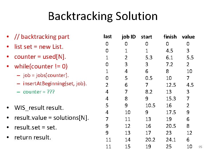
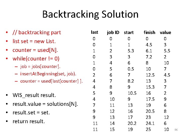
Backtracking Solution • • // backtracking part list set = new List. counter = used[N]. while(counter != 0) – job = jobs[counter]. – insert. At. Beginning(set, job). – counter = ? ? ? • • WIS_result. value = solutions[N]. result. set = set. return result. last 0 0 1 0 2 4 4 5 4 7 9 9 11 11 job ID start 0 0 1 1 2 5. 3 3 3 4 6 5 0. 5 6 7 7 8. 2 8 9 9 10. 5 10 9 11 13 12 16 13 17 14 20. 2 15 19 finish value 0 0 4. 5 3 6. 1 5. 5 7. 2 2 8 10 10 7 12. 5 4. 5 13 3 15. 3 7 16 2 17. 5 9 19 6 20. 5 8 23 12 24. 1 6 25 10 95

Backtracking Solution • • // backtracking part list set = new List. counter = used[N]. while(counter != 0) – job = jobs[counter]. – insert. At. Beginning(set, job). – counter = used[last[counter] ]. • • WIS_result. value = solutions[N]. result. set = set. return result. last 0 0 1 0 2 4 4 5 4 7 9 9 11 11 job ID start 0 0 1 1 2 5. 3 3 3 4 6 5 0. 5 6 7 7 8. 2 8 9 9 10. 5 10 9 11 13 12 16 13 17 14 20. 2 15 19 finish value 0 0 4. 5 3 6. 1 5. 5 7. 2 2 8 10 10 7 12. 5 4. 5 13 3 15. 3 7 16 2 17. 5 9 19 6 20. 5 8 23 12 24. 1 6 25 10 96

Matrix Multiplication: Review • Suppose that A 1 is of size S 1 x S 2, and A 2 is of size S 2 x S 3. • What is the time complexity of computing A 1 * A 2? • What is the size of the result? 97

Matrix Multiplication: Review • Suppose that A 1 is of size S 1 x S 2, and A 2 is of size S 2 x S 3. • What is the time complexity of computing A 1 * A 2? • What is the size of the result? S 1 x S 3. • Each number in the result is computed in O(S 2) time by: – multiplying S 2 pairs of numbers. – adding S 2 numbers. • Overall time complexity: O(S 1 * S 2 * S 3). 98

Optimal Ordering for Matrix Multiplication • Suppose that we need to do a sequence of matrix multiplications: – result = A 1 * A 2 * A 3 *. . . * AK • The number of columns for Ai must equal the number of rows for Ai+1. • What is the time complexity for performing this sequence of multiplications? 99

Optimal Ordering for Matrix Multiplication • Suppose that we need to do a sequence of matrix multiplications: – result = A 1 * A 2 * A 3 *. . . * AK • The number of columns for Ai must equal the number of rows for Ai+1. • What is the time complexity for performing this sequence of multiplications? • The answer is: it depends on the order in which we perform the multiplications. 100

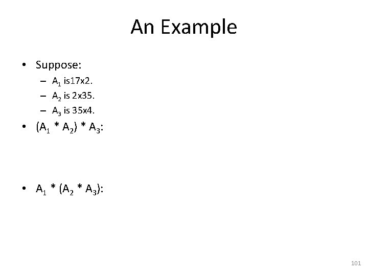
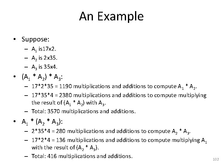
An Example • Suppose: – A 1 is 17 x 2. – A 2 is 2 x 35. – A 3 is 35 x 4. • (A 1 * A 2) * A 3: • A 1 * (A 2 * A 3): 101

An Example • Suppose: – A 1 is 17 x 2. – A 2 is 2 x 35. – A 3 is 35 x 4. • (A 1 * A 2) * A 3: – 17*2*35 = 1190 multiplications and additions to compute A 1 * A 2. – 17*35*4 = 2380 multiplications and additions to compute multiplying the result of (A 1 * A 2) with A 3. – Total: 3570 multiplications and additions. • A 1 * (A 2 * A 3): – 2*35*4 = 280 multiplications and additions to compute A 2 * A 3. – 17*2*4 = 136 multiplications and additions to compute multiplying A 1 with the result of (A 2 * A 3). – Total: 416 multiplications and additions. 102

Adaptation to Dynamic Programming • Suppose that we need to do a sequence of matrix multiplications: – result = A 1 * A 2 * A 3 *. . . * AK • To figure out if and how we can use dynamic programming, we must address the standard two questions we always need to address for dynamic programming: 1. Can we define a set of smaller problems, such that the solutions to those problems make it easy to solve the original problem? 2. Can we arrange those smaller problems in a sequence of reasonable size, so that each problem in that sequence only depends on problems that come earlier in the sequence? 103

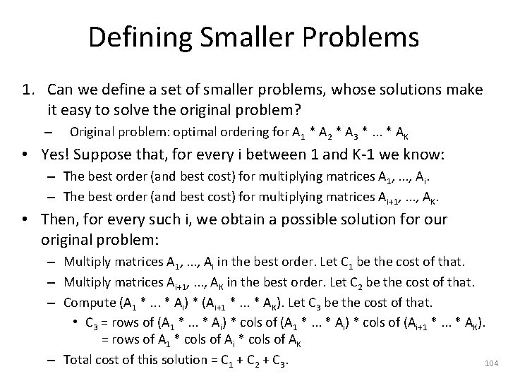
Defining Smaller Problems 1. Can we define a set of smaller problems, whose solutions make it easy to solve the original problem? – Original problem: optimal ordering for A 1 * A 2 * A 3 *. . . * AK • Yes! Suppose that, for every i between 1 and K-1 we know: – The best order (and best cost) for multiplying matrices A 1, . . . , Ai. – The best order (and best cost) for multiplying matrices Ai+1, . . . , AK. • Then, for every such i, we obtain a possible solution for our original problem: – Multiply matrices A 1, . . . , Ai in the best order. Let C 1 be the cost of that. – Multiply matrices Ai+1, . . . , AK in the best order. Let C 2 be the cost of that. – Compute (A 1 *. . . * Ai) * (Ai+1 *. . . * AK). Let C 3 be the cost of that. • C 3 = rows of (A 1 *. . . * Ai) * cols of (Ai+1 *. . . * AK). = rows of A 1 * cols of Ai * cols of AK – Total cost of this solution = C 1 + C 2 + C 3. 104

Defining Smaller Problems 1. Can we define a set of smaller problems, whose solutions make it easy to solve the original problem? – Original problem: optimal ordering for A 1 * A 2 * A 3 *. . . * AK • Yes! Suppose that, for every i between 1 and K-1 we know: – The best order (and best cost) for multiplying matrices A 1, . . . , Ai. – The best order (and best cost) for multiplying matrices Ai+1, . . . , AK. • Then, for every such i, we obtain a possible solution. • We just need to compute the cost of each of those solutions, and choose the smallest cost. • Next question: 2. Can we arrange those smaller problems in a sequence of reasonable size, so that each problem in that sequence only depends on problems that come earlier in the sequence? 105

Defining Smaller Problems 2. Can we arrange those smaller problems in a sequence of reasonable size, so that each problem in that sequence only depends on problems that come earlier in the sequence? • To compute answer for A 1 * A 2 * A 3 *. . . * AK : For i = 1, …, K-1, we had to consider solutions for: – A 1, . . . , Ai. – Ai+1, . . . , AK. • So, what is the set of all problems we must solve? 106

Defining Smaller Problems 2. Can we arrange those smaller problems in a sequence of reasonable size, so that each problem in that sequence only depends on problems that come earlier in the sequence? • To compute answer for A 1 * A 2 * A 3 *. . . * AK : For i = 1, …, K-1, we had to consider solutions for: – A 1, . . . , Ai. – Ai+1, . . . , AK. • So, what is the set of all problems we must solve? • For M = 1, . . . , K. – For N = 1, . . . , M. • Compute the best ordering for AN *. . . * AM. • What this the number of problems we need to solve? Is the size reasonable? – We must solve Θ(K 2) problems. We consider this a reasonable number. 107

Defining Smaller Problems • The set of all problems we must solve: • For M = 1, . . . , K. – For N = 1, . . . , M. • Compute the best ordering for AN *. . . * AM. • What is the order in which we must solve these problems? 108

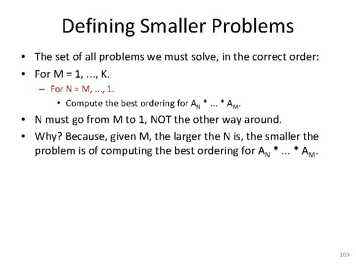
Defining Smaller Problems • The set of all problems we must solve, in the correct order: • For M = 1, . . . , K. – For N = M, . . . , 1. • Compute the best ordering for AN *. . . * AM. • N must go from M to 1, NOT the other way around. • Why? Because, given M, the larger the N is, the smaller the problem is of computing the best ordering for AN *. . . * AM. 109

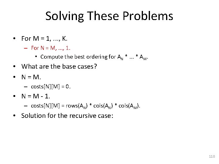
Solving These Problems • For M = 1, . . . , K. – For N = M, . . . , 1. • Compute the best ordering for AN *. . . * AM. • What are the base cases? • N = M. – costs[N][M] = 0. • N = M - 1. – costs[N][M] = rows(AN) * cols(AM). • Solution for the recursive case: 110

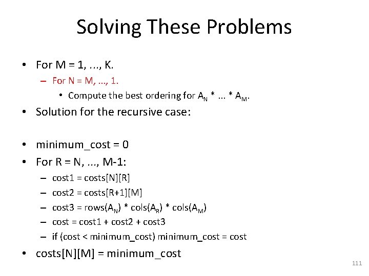
Solving These Problems • For M = 1, . . . , K. – For N = M, . . . , 1. • Compute the best ordering for AN *. . . * AM. • Solution for the recursive case: • minimum_cost = 0 • For R = N, . . . , M-1: – – – cost 1 = costs[N][R] cost 2 = costs[R+1][M] cost 3 = rows(AN) * cols(AR) * cols(AM) cost = cost 1 + cost 2 + cost 3 if (cost < minimum_cost) minimum_cost = cost • costs[N][M] = minimum_cost 111

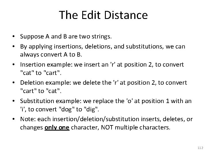
The Edit Distance • Suppose A and B are two strings. • By applying insertions, deletions, and substitutions, we can always convert A to B. • Insertion example: we insert an 'r' at position 2, to convert "cat" to "cart". • Deletion example: we delete the 'r' at position 2, to convert "cart" to "cat". • Substitution example: we replace the 'o' at position 1 with an 'i', to convert "dog" to "dig". • Note: each insertion/deletion/substitution inserts, deletes, or changes only one character, NOT multiple characters. 112

The Edit Distance • For example, to convert "chicken" to "ticket": • One solution: – – Substitute 'c' with 't'. Delete 'h'. Replace 'n' with 't'. Total: three operations. • Another solution: – – Delete 'c'. Substitute 'h' with 't'. Replace 'n' with 't'. Total: three operations. 113

The Edit Distance • Question: given two strings A and B, what is the smallest number of operations we need in order to convert A to B? • The answer is called the edit distance between A and B. • This distance, and variations, have significant applications in various fields, including bioinformatics and pattern recognition. 114

Visualizing the Edit Distance • Assignment preview: you will have to write code that produces such output. • Edit distance between "chicken" and "ticket" = ? 115

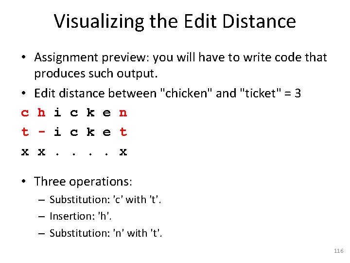
Visualizing the Edit Distance • Assignment preview: you will have to write code that produces such output. • Edit distance between "chicken" and "ticket" = 3 c h i c k e n t - i c k e t x x. . x • Three operations: – Substitution: 'c' with 't'. – Insertion: 'h'. – Substitution: 'n' with 't'. 116

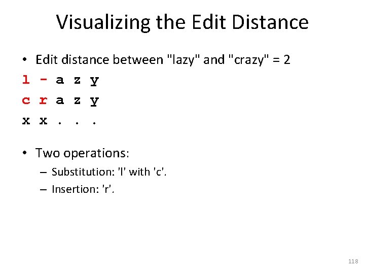
Visualizing the Edit Distance • Edit distance between "lazy" and "crazy" = ? 117

Visualizing the Edit Distance • l c x Edit distance between "lazy" and "crazy" = 2 - a z y r a z y x. . . • Two operations: – Substitution: 'l' with 'c'. – Insertion: 'r'. 118

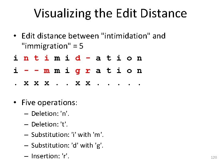
Visualizing the Edit Distance • Edit distance between "intimidation" and "immigration" = ? 119

Visualizing the Edit Distance • Edit distance between "intimidation" and "immigration" = 5 i n t i m i d - a t i o n i - - m m i g r a t i o n. x x x. . • Five operations: – – – Deletion: 'n'. Deletion: 't'. Substitution: 'i' with 'm'. Substitution: 'd' with 'g'. Insertion: 'r'. 120

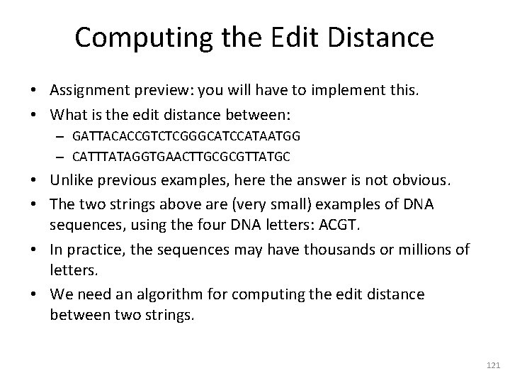
Computing the Edit Distance • Assignment preview: you will have to implement this. • What is the edit distance between: – GATTACACCGTCTCGGGCATCCATAATGG – CATTTATAGGTGAACTTGCGCGTTATGC • Unlike previous examples, here the answer is not obvious. • The two strings above are (very small) examples of DNA sequences, using the four DNA letters: ACGT. • In practice, the sequences may have thousands or millions of letters. • We need an algorithm for computing the edit distance between two strings. 121

Computing the Edit Distance • To find a dynamic programming solution, we must find a sequence of problems such that: – Each problem in the sequence can be easily solved given solutions to the previous problems. – The number of problems in the sequence is not too large (e. g. , not exponential). • Any ideas? • Given strings A and B, can you identify smaller problems that are related to computing the edit distance between A and B? 122

Computing the Edit Distance • Notation: – S[i, . . . , j] is the substring of S that includes all letters from position i to position j. – |S| indicates the length of string S. • Using this notation: – A = A[0, . . . , |A|-1] – B = B[0, . . . , |B|-1] • The solution for edit_distance(A, B) depends on the solutions to three smaller problems: – edit_distance(A[0, . . . , |A|-1], B[0, . . . , |B|-2]) – edit_distance(A[0, . . . , |A|-2], B[0, . . . , |B|-1]) – edit_distance(A[0, . . . , |A|-2], B[0, . . . , |B|-2]) 123

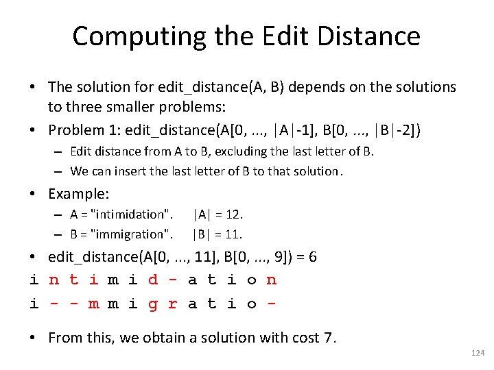
Computing the Edit Distance • The solution for edit_distance(A, B) depends on the solutions to three smaller problems: • Problem 1: edit_distance(A[0, . . . , |A|-1], B[0, . . . , |B|-2]) – Edit distance from A to B, excluding the last letter of B. – We can insert the last letter of B to that solution. • Example: – A = "intimidation". – B = "immigration". |A| = 12. |B| = 11. • edit_distance(A[0, . . . , 11], B[0, . . . , 9]) = 6 i n t i m i d - a t i o n i - - m m i g r a t i o • From this, we obtain a solution with cost 7. 124

Computing the Edit Distance • Problem 2: edit_distance(A[0, . . . , |A|-2], B[0, . . . , |B|-1]) – Edit distance from A to B, excluding the last letter of A. – We can insert the last letter of A to that solution. • Example: – A = "intimidation". – B = "immigration". |A| = 12. |B| = 11. • edit_distance(A[0, . . . , 10], B[0, . . . , 10]) = 6 i n t i m i d - a t i o i - - m m i g r a t i o n • This solution converts "intimidatio" to "immigration". • Using one more deletion (of the final 'n' of "intimidation"), we convert "intimidation" to "immigration" with cost 7. 125

Computing the Edit Distance • Problem 3: edit_distance(A[0, . . . , |A|-2], B[0, . . . , |B|-2]) – Edit distance from A to B, excluding the last letter of both A and B. • Example: – A = "intimidation". – B = "immigration". |A| = 12. |B| = 11. • edit_distance(A[0, . . . , 10], B[0, . . . , 9]) = 5 i n t i m i d - a t i o i - - m m i g r a t i o • This solution converts "intimidatio" to "immigratio". • The same solution converts "intimidation" to "immigration", because both words have the same last letter. 126

Computing the Edit Distance • Problem 3: edit_distance(A[0, . . . , |A|-2], B[0, . . . , |B|-2]) – Edit distance from A to B, excluding the last letter of both A and B. • Example: – A = "nation". – B = "patios". |A| = 6. |B| = 6. • edit_distance(A[0, . . . , 10], B[0, . . . , 9]) = 1 n a t i o p a t i o • This solution converts "natio" to " patio". • The same solution, plus one substitution ('n' with 's') converts "nation" to "patios", with cost 2. 127

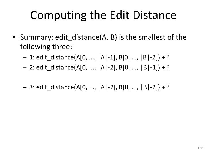
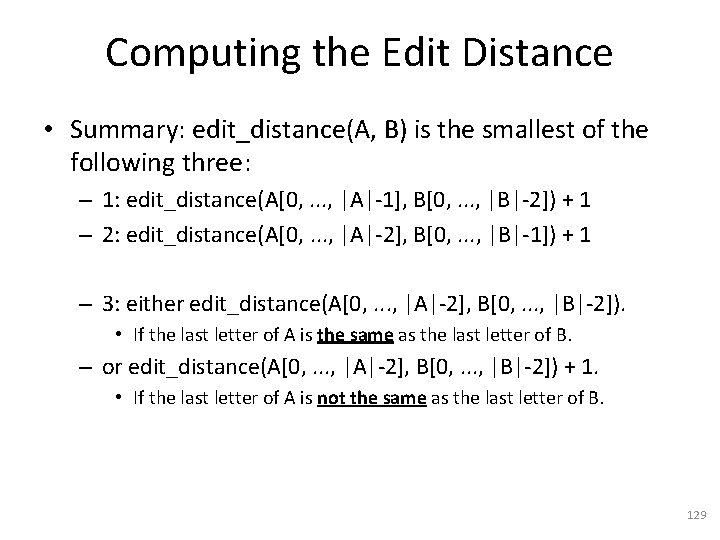
Computing the Edit Distance • Summary: edit_distance(A, B) is the smallest of the following three: – 1: edit_distance(A[0, . . . , |A|-1], B[0, . . . , |B|-2]) + ? – 2: edit_distance(A[0, . . . , |A|-2], B[0, . . . , |B|-1]) + ? – 3: edit_distance(A[0, . . . , |A|-2], B[0, . . . , |B|-2]) + ? 128

Computing the Edit Distance • Summary: edit_distance(A, B) is the smallest of the following three: – 1: edit_distance(A[0, . . . , |A|-1], B[0, . . . , |B|-2]) + 1 – 2: edit_distance(A[0, . . . , |A|-2], B[0, . . . , |B|-1]) + 1 – 3: either edit_distance(A[0, . . . , |A|-2], B[0, . . . , |B|-2]). • If the last letter of A is the same as the last letter of B. – or edit_distance(A[0, . . . , |A|-2], B[0, . . . , |B|-2]) + 1. • If the last letter of A is not the same as the last letter of B. 129

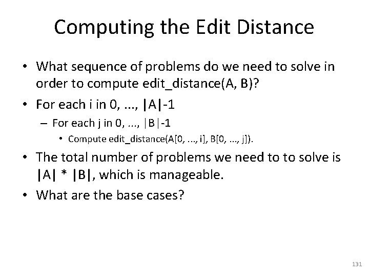
Computing the Edit Distance • What sequence of problems do we need to solve in order to compute edit_distance(A, B)? 130

Computing the Edit Distance • What sequence of problems do we need to solve in order to compute edit_distance(A, B)? • For each i in 0, . . . , |A|-1 – For each j in 0, . . . , |B|-1 • Compute edit_distance(A[0, . . . , i], B[0, . . . , j]). • The total number of problems we need to to solve is |A| * |B|, which is manageable. • What are the base cases? 131

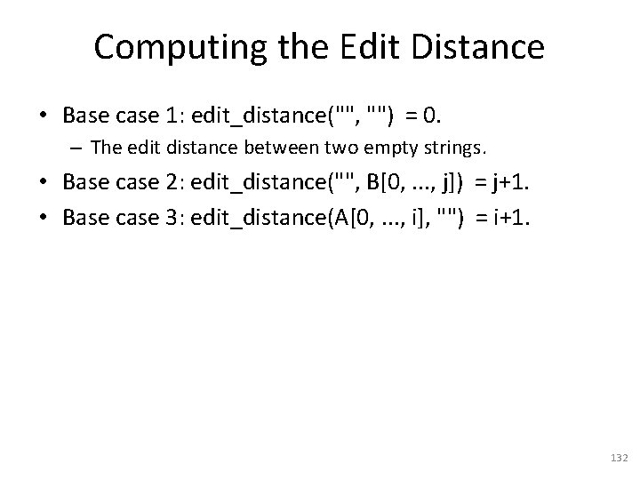
Computing the Edit Distance • Base case 1: edit_distance("", "") = 0. – The edit distance between two empty strings. • Base case 2: edit_distance("", B[0, . . . , j]) = j+1. • Base case 3: edit_distance(A[0, . . . , i], "") = i+1. 132

Computing the Edit Distance • For convenience, we define A[0, -1] = "", B[0, -1] = "". • Then, we can rewrite the previous base cases like this: • Base case 1: edit_distance(A[0, -1], B[0, -1]) = 0. – The edit distance between two empty strings. • Base case 2: edit_distance(A[0, -1], B[0, . . . , j]) = j+1. • Base case 3: edit_distance(A[0, . . . , i], B[0, -1]) = i+1. 133

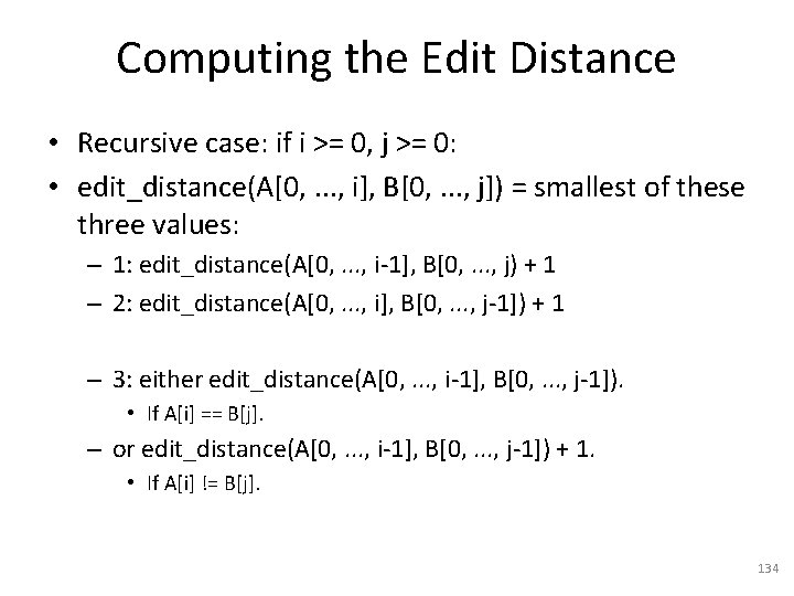
Computing the Edit Distance • Recursive case: if i >= 0, j >= 0: • edit_distance(A[0, . . . , i], B[0, . . . , j]) = smallest of these three values: – 1: edit_distance(A[0, . . . , i-1], B[0, . . . , j) + 1 – 2: edit_distance(A[0, . . . , i], B[0, . . . , j-1]) + 1 – 3: either edit_distance(A[0, . . . , i-1], B[0, . . . , j-1]). • If A[i] == B[j]. – or edit_distance(A[0, . . . , i-1], B[0, . . . , j-1]) + 1. • If A[i] != B[j]. 134