RECONSTRUCTION OF REMOTE SENSING TIME SERIES DATA Javier

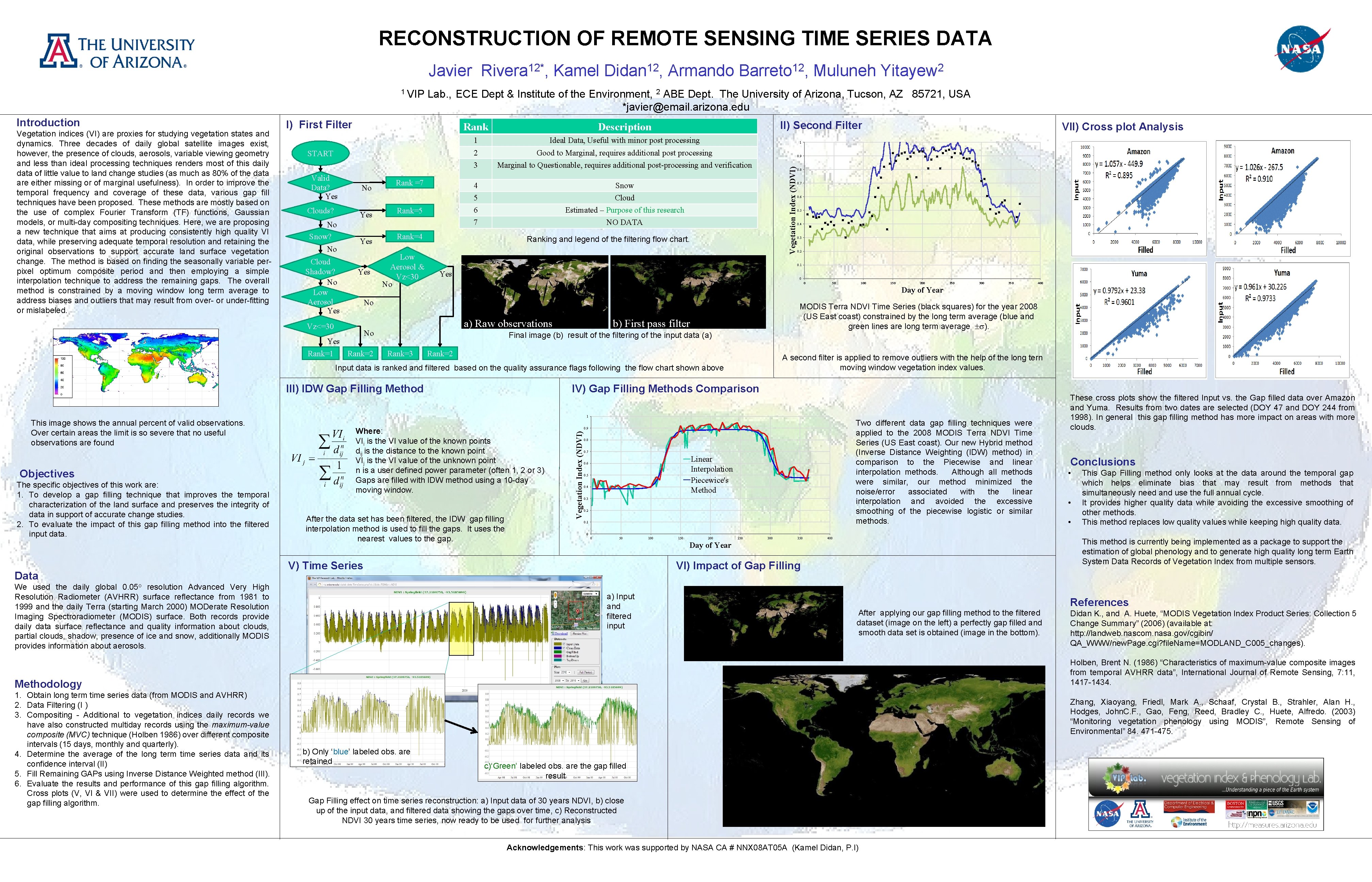
RECONSTRUCTION OF REMOTE SENSING TIME SERIES DATA Javier Introduction Vegetation indices (VI) are proxies for studying vegetation states and dynamics. Three decades of daily global satellite images exist, however, the presence of clouds, aerosols, variable viewing geometry and less than ideal processing techniques renders most of this daily data of little value to land change studies (as much as 80% of the data are either missing or of marginal usefulness). In order to improve the temporal frequency and coverage of these data, various gap fill techniques have been proposed. These methods are mostly based on the use of complex Fourier Transform (TF) functions, Gaussian models, or multi-day compositing techniques. Here, we are proposing a new technique that aims at producing consistently high quality VI data, while preserving adequate temporal resolution and retaining the original observations to support accurate land surface vegetation change. The method is based on finding the seasonally variable perpixel optimum composite period and then employing a simple interpolation technique to address the remaining gaps. The overall method is constrained by a moving window long term average to address biases and outliers that may result from over- or under-fitting or mislabeled. START Clouds? No Yes No Snow? No Cloud Shadow? No Low Aerosol Yes Yes Rank =7 Rank=5 Description 1 Ideal Data, Useful with minor post processing 2 Good to Marginal, requires additional post processing 3 Marginal to Questionable, requires additional post-processing and verification 4 5 6 Snow Cloud Estimated – Purpose of this research 7 NO DATA 0. 9 Ranking and legend of the filtering flow chart. Yes Data 0. 4 0. 3 0. 2 50 Final image (b) result of the filtering of the input data (a) Rank=2 200 250 300 350 400 IV) Gap Filling Methods Comparison Where: VIi is the VI value of the known points dij is the distance to the known point VIj is the VI value of the unknown point n is a user defined power parameter (often 1, 2 or 3) Gaps are filled with IDW method using a 10 -day moving window. After the data set has been filtered, the IDW gap filling interpolation method is used to fill the gaps. It uses the nearest values to the gap. Two different data gap filling techniques were applied to the 2008 MODIS Terra NDVI Time Series (US East coast). Our new Hybrid method (Inverse Distance Weighting (IDW) method) in comparison to the Piecewise and linear interpolation methods. Although all methods were similar, our method minimized the noise/error associated with the linear interpolation and avoided the excessive smoothing of the piecewise logistic or similar methods. 0. 9 0. 8 0. 7 Linear Interpolation Piecewice's Method 0. 6 0. 5 0. 4 0. 3 0. 2 0. 1 These cross plots show the filtered Input vs. the Gap filled data over Amazon and Yuma. Results from two dates are selected (DOY 47 and DOY 244 from 1998). In general this gap filling method has more impact on areas with more clouds. Conclusions • • • This Gap Filling method only looks at the data around the temporal gap which helps eliminate bias that may result from methods that simultaneously need and use the full annual cycle. It provides higher quality data while avoiding the excessive smoothing of other methods. This method replaces low quality values while keeping high quality data. 0 0 50 100 150 200 250 300 350 400 This method is currently being implemented as a package to support the estimation of global phenology and to generate high quality long term Earth System Data Records of Vegetation Index from multiple sensors. Day of Year V) Time Series VI) Impact of Gap Filling a) Input and filtered input After applying our gap filling method to the filtered dataset (image on the left) a perfectly gap filled and smooth data set is obtained (image in the bottom). References Didan K. , and A. Huete, “MODIS Vegetation Index Product Series: Collection 5 Change Summary” (2006) (available at: http: //landweb. nascom. nasa. gov/cgibin/ QA_WWW/new. Page. cgi? file. Name=MODLAND_C 005_changes). Holben, Brent N. (1986) “Characteristics of maximum-value composite images from temporal AVHRR data”, International Journal of Remote Sensing, 7: 11, 1417 -1434. Methodology 1. Obtain long term time series data (from MODIS and AVHRR) 2. Data Filtering (I ) 3. Compositing - Additional to vegetation indices daily records we have also constructed multiday records using the maximum-value composite (MVC) technique (Holben 1986) over different composite intervals (15 days, monthly and quarterly). 4. Determine the average of the long term time series data and its confidence interval (II) 5. Fill Remaining GAPs using Inverse Distance Weighted method (III). 6. Evaluate the results and performance of this gap filling algorithm. Cross plots (V, VI & VII) were used to determine the effect of the gap filling algorithm. 150 A second filter is applied to remove outliers with the help of the long tern moving window vegetation index values. 1 We used the daily global 0. 05 o resolution Advanced Very High Resolution Radiometer (AVHRR) surface reflectance from 1981 to 1999 and the daily Terra (starting March 2000) MODerate Resolution Imaging Spectroradiometer (MODIS) surface. Both records provide daily data surface reflectance and quality information about clouds, partial clouds, shadow, presence of ice and snow, additionally MODIS provides information about aerosols. 100 MODIS Terra NDVI Time Series (black squares) for the year 2008 (US East coast) constrained by the long term average (blue and green lines are long term average ). b) First pass filter Vegetation Index (NDVI) The specific objectives of this work are: 1. To develop a gap filling technique that improves the temporal characterization of the land surface and preserves the integrity of data in support of accurate change studies. 2. To evaluate the impact of this gap filling method into the filtered input data. 0. 5 Day of Year III) IDW Gap Filling Method Objectives 0. 6 0 Input data is ranked and filtered based on the quality assurance flags following the flow chart shown above This image shows the annual percent of valid observations. Over certain areas the limit is so severe that no useful observations are found 0. 7 0 a) Raw observations Rank=3 0. 8 0. 1 No Yes Rank=1 Rank=2 VII) Cross plot Analysis 1 No Vz<=30 Muluneh 2 Yitayew II) Second Filter Rank=4 Low Aerosol & Vz<30 No Armando 12 Barreto , Lab. , ECE Dept & Institute of the Environment, 2 ABE Dept. The University of Arizona, Tucson, AZ 85721, USA *javier@email. arizona. edu I) First Filter Valid Data? Yes Kamel 12 Didan , Vegetation Index (NDVI) 1 VIP 12* Rivera , Zhang, Xiaoyang, Friedl, Mark A. , Schaaf, Crystal B. , Strahler, Alan H. , Hodges, John. C. F. , Gao, Feng, Reed, Bradley C. , Huete, Alfredo. (2003) “Monitoring vegetation phenology using MODIS”, Remote Sensing of Environmental” 84. 471 -475. b) Only ‘blue’ labeled obs. are retained c)‘Green’ labeled obs. are the gap filled result Gap Filling effect on time series reconstruction: a) Input data of 30 years NDVI, b) close up of the input data, and filtered data showing the gaps over time, c) Reconstructed NDVI 30 years time series, now ready to be used for further analysis Acknowledgements: This work was supported by NASA CA # NNX 08 AT 05 A (Kamel Didan, P. I)