Reconstructing Relief Surfaces George Vogiatzis Philip Torr Steven

Reconstructing Relief Surfaces George Vogiatzis, Philip Torr, Steven Seitz and Roberto Cipolla BMVC 2004

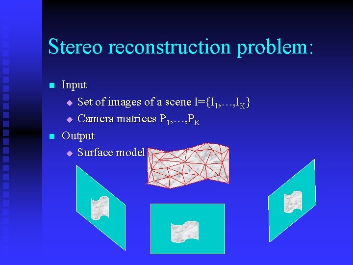
Stereo reconstruction problem: n n Input u Set of images of a scene I={I 1, …, IK} u Camera matrices P 1, …, PK Output u Surface model

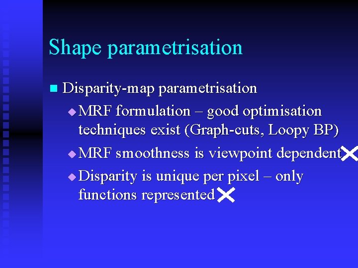
Shape parametrisation n Disparity-map parametrisation u MRF formulation – good optimisation techniques exist (Graph-cuts, Loopy BP) u MRF smoothness is viewpoint dependent u Disparity is unique per pixel – only functions represented

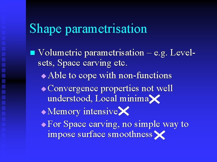
Shape parametrisation n Volumetric parametrisation – e. g. Levelsets, Space carving etc. u Able to cope with non-functions u Convergence properties not well understood, Local minima u Memory intensive u For Space carving, no simple way to impose surface smoothness

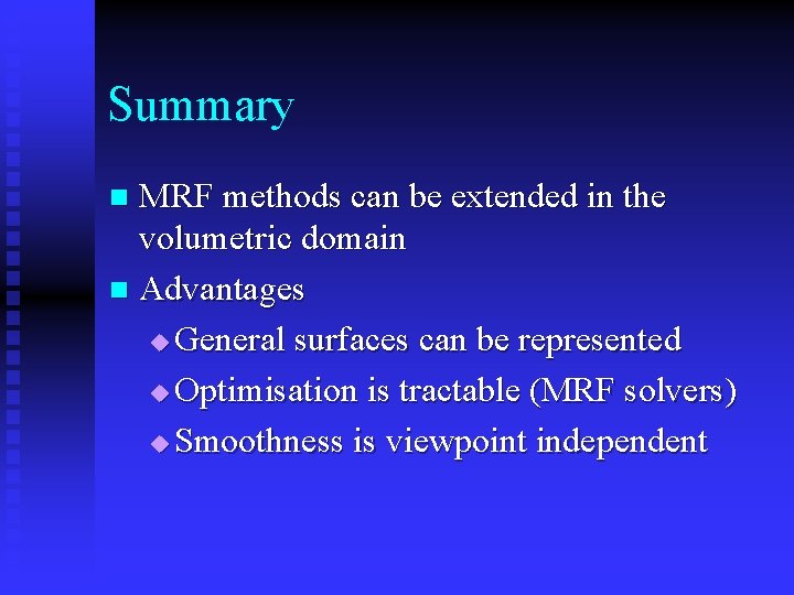
Solution ? n n n Cast volumetric methods in MRF framework Key assumption: Approximate scene geometry given Benefits: u General surfaces can be represented u Optimisation is tractable (MRF solvers) u Occlusions are approximately modelled u Smoothness is viewpoint independent

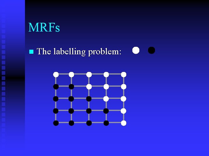
MRFs n The labelling problem:

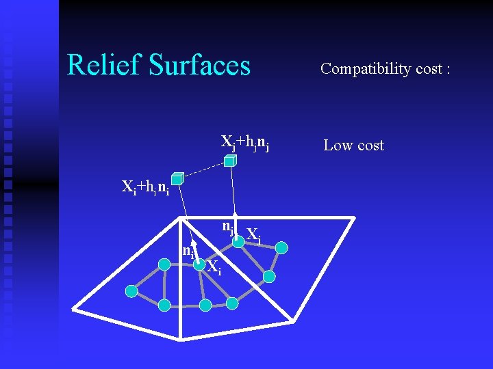
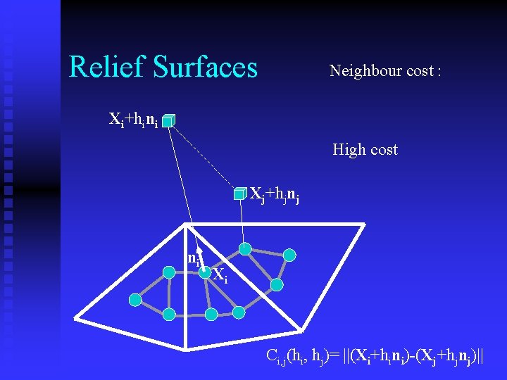
MRFs n n n A set of random variables h 1, …, h. M A binary neighbourhood relation N defined on the variables Each can take a label out of a set H 1, …, HL Ci(hi) (Labelling cost) Ci, j(hi, hj) for (i, j) N (Compatibility cost) -log P(h 1, …, h. M) = Ci(hi) + Ci, j(hi, hj)

MRF inference Minimise Ci(hi) + Ci, j(hi, hj) n Not in polynomial time in general case n Special cases (e. g. no loops or 2 label MRF) solved exactly n General cases solved approximately via Graph-cuts or Loopy Belief Propagation. Approx. 10 -15 mins for MRF with 250, 000 nodes. n

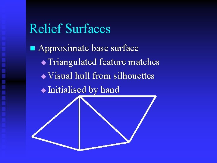
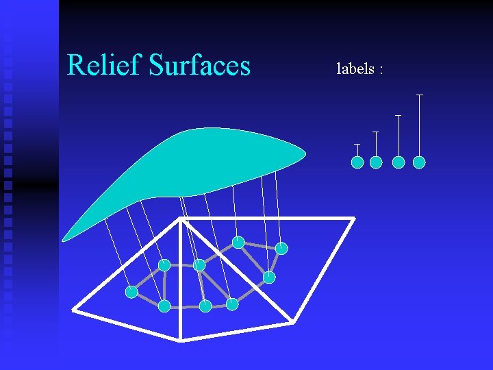
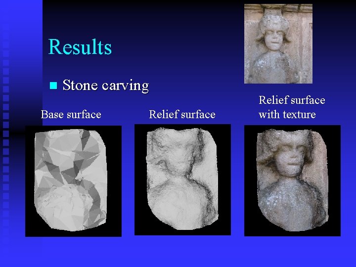
Relief Surfaces n Approximate base surface u Triangulated feature matches u Visual hull from silhouettes u Initialised by hand

Relief Surfaces labels :

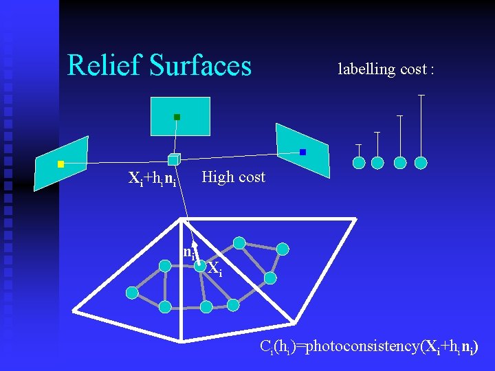
Relief Surfaces labelling cost : Low cost High cost Xi+hini ni Xi Ci(hi)=photoconsistency(Xi+hini)

Relief Surfaces Xj+hjnj Xi+hini nj ni Xi Xj Compatibility cost : Low cost

Relief Surfaces Neighbour cost : Xi+hini High cost Xj+hjnj ni Xi Ci, j(hi, hj)= ||(Xi+hini)-(Xj+hjnj)||

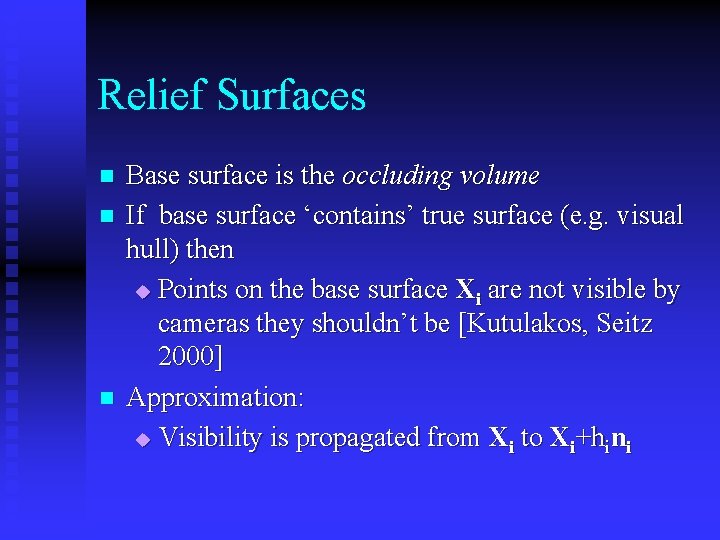
Relief Surfaces n n n Base surface is the occluding volume If base surface ‘contains’ true surface (e. g. visual hull) then u Points on the base surface Xi are not visible by cameras they shouldn’t be [Kutulakos, Seitz 2000] Approximation: u Visibility is propagated from Xi to Xi+hini

Loopy Belief Propagation min Ci(hi) + Ci, j(hi, hj) n n Iterative message passing algorithm m(t)i, j (hj) is the message passed from i to j at time step t It is a L-dimensional vector Represents what node i ‘believes’ about the true state of node j. i mi, j j

Loopy Belief Propagation n Message passing rule: m(t+1)i, j (hj)= min{ Cij(hi, hj) +Ci(hi) + m(t)k, i (hi)} k N(i) hi n After convergence, optimal state is given by hi*= min{Ci(hi) + m( )k, i (hi)} hi k N(i) i mi, j j

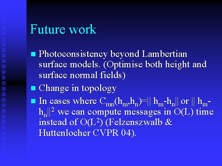
Loopy Belief Propagation O(L 2) to compute a message (L is number of allowable heights) n Message passing schedule can be asynchronous which can accelerate convergence [Tappen & Freeman ICCV 03] n

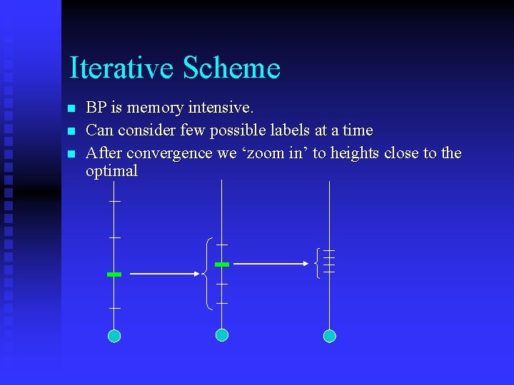
Iterative Scheme n n n BP is memory intensive. Can consider few possible labels at a time After convergence we ‘zoom in’ to heights close to the optimal

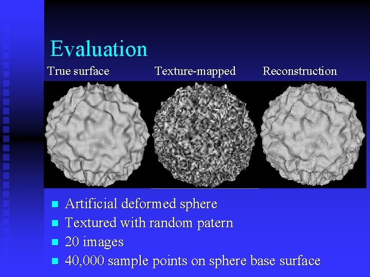
Evaluation True surface n n Texture-mapped Reconstruction Artificial deformed sphere Textured with random patern 20 images 40, 000 sample points on sphere base surface

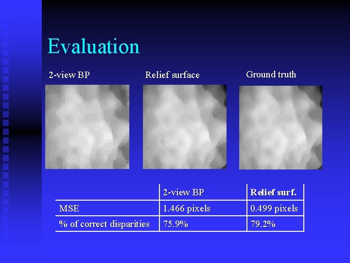
Evaluation Benchmark: 2 -view, disparity based Loopy Belief Propagation [Sun et al ECCV 02] n BP run on 10 pairs of nearby views n Compare Disparity Maps given by u 2 -view BP u Relief surfaces u Ground truth n

Evaluation 2 -view BP Relief surface Ground truth 2 -view BP Relief surf. MSE 1. 466 pixels 0. 499 pixels % of correct disparities 75. 9% 79. 2%

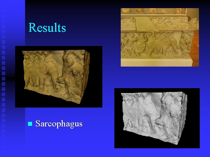
Results n Sarcophagus

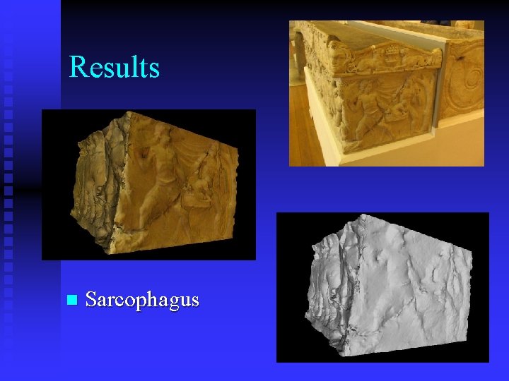
Results n Sarcophagus

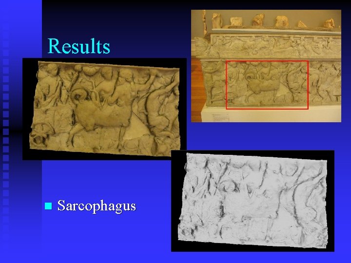
Results n Sarcophagus

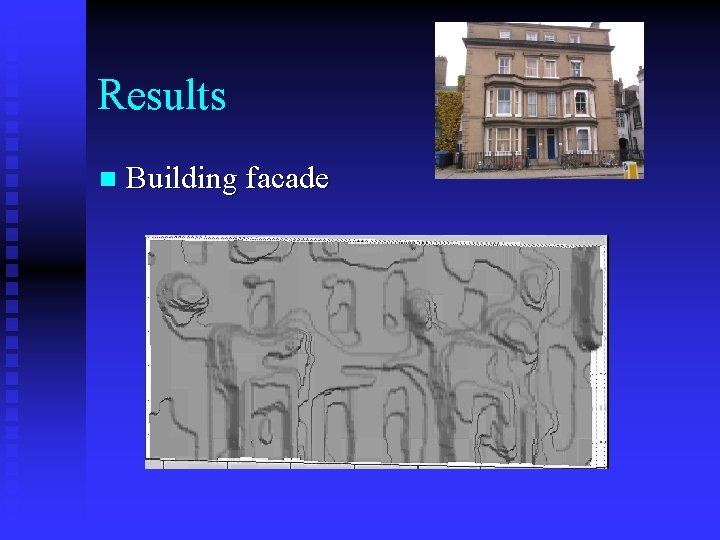
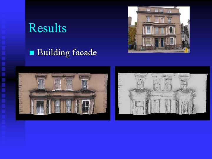
Results n Building facade

Results n Building facade

Results n Stone carving Base surface Relief surface with texture

Summary MRF methods can be extended in the volumetric domain n Advantages u General surfaces can be represented u Optimisation is tractable (MRF solvers) u Smoothness is viewpoint independent n

Future work Photoconsistency beyond Lambertian surface models. (Optimise both height and surface normal fields) n Change in topology n In cases where Cmn(hm, hn)=|| hm-hn|| or || hmhn||2 we can compute messages in O(L) time instead of O(L 2) (Felzenszwalb & Huttenlocher CVPR 04). n