Recognition SVD and PCA Recognition Suppose you want
- Slides: 29

Recognition, SVD, and PCA

Recognition • Suppose you want to find a face in an image • One possibility: look for something that looks sort of like a face (oval, dark band near top, dark band near bottom) • Another possibility: look for pieces of faces (eyes, mouth, etc. ) in a specific arrangement

Templates • Model of a “generic” or “average” face – Learn templates from example data • For each location in image, look for template at that location – Optionally also search over scale, orientation

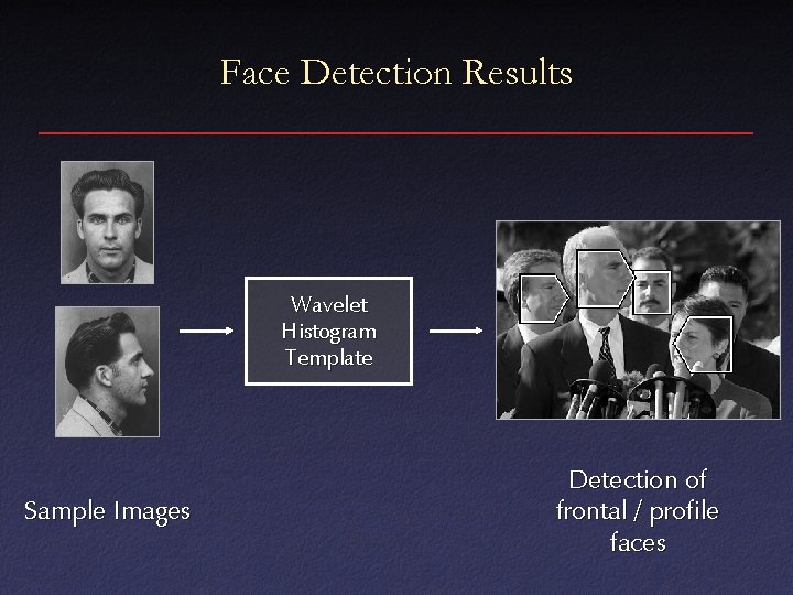
Templates • In the simplest case, based on intensity – Template is average of all faces in training set – Comparison based on e. g. SSD • More complex templates – Outputs of feature detectors – Color histograms – Both position and frequency information (wavelets)

Face Detection Results Wavelet Histogram Template Sample Images Detection of frontal / profile faces

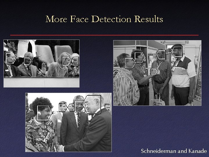
More Face Detection Results Schneiderman and Kanade

Recognition Using Relations Between Templates • Often easier to recognize a small feature – e. g. , lips easier to recognize than faces – For articulated objects (e. g. people), template for whole class usually complicated • So, identify small pieces and look for spatial arrangements – Many false positives from identifying pieces

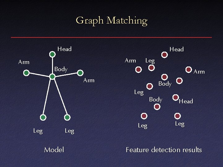
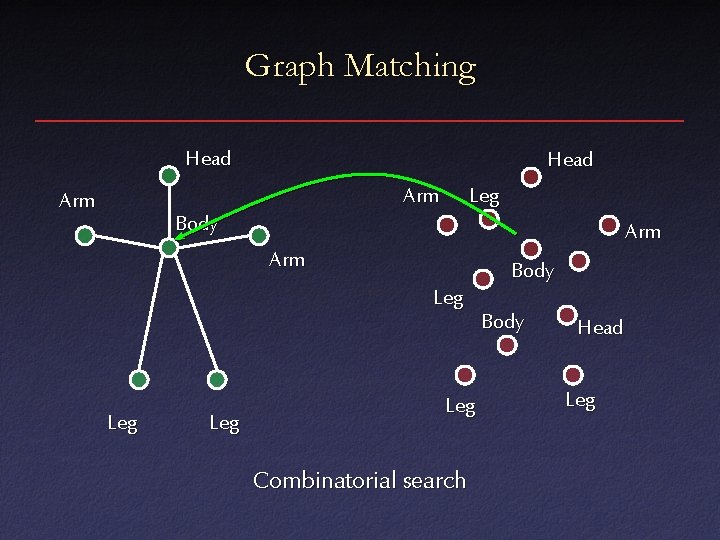
Graph Matching Head Arm Leg Body Arm Body Leg Leg Model Leg Body Head Leg Feature detection results

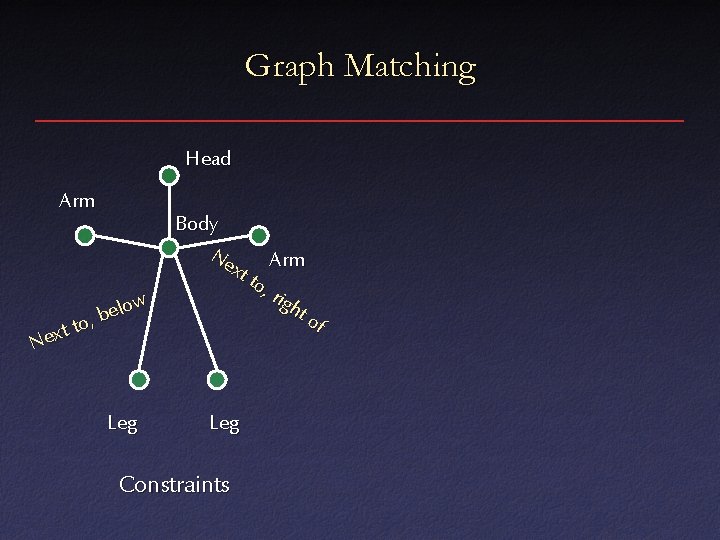
Graph Matching Head Arm low e b , o t t Nex Leg Body Ne xt Arm to, rig ht of Leg Constraints

Graph Matching Head Arm Leg Body Arm Body Leg Leg Combinatorial search Body Head Leg

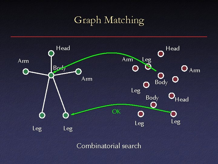
Graph Matching Head Arm Leg Body Arm Body Leg Body Head OK Leg Leg Combinatorial search Leg

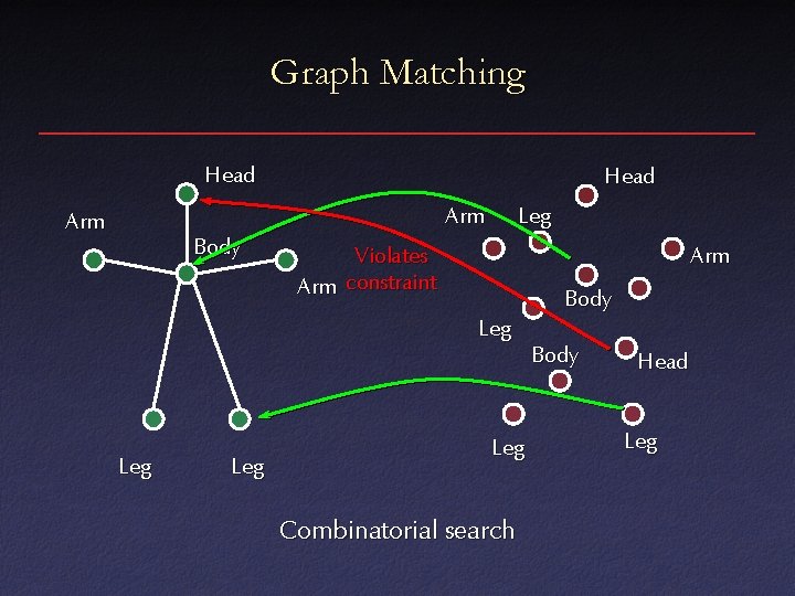
Graph Matching Head Arm Body Leg Violates Arm constraint Arm Body Leg Leg Combinatorial search Body Head Leg

Graph Matching • Large search space – Heuristics for pruning • Missing features – Look for maximal consistent assignment • Noise, spurious features • Incomplete constraints – Verification step at end

Recognition • Suppose you want to recognize a particular face • How does this face differ from average face

How to Recognize Specific People? • Consider variation from average face • Not all variations equally important – Variation in a single pixel relatively unimportant • If image is high-dimensional vector, want to find directions in this space with high variation

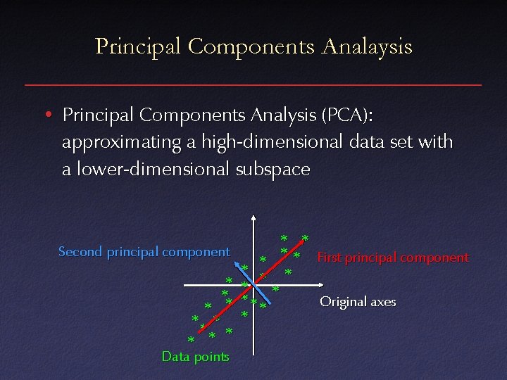
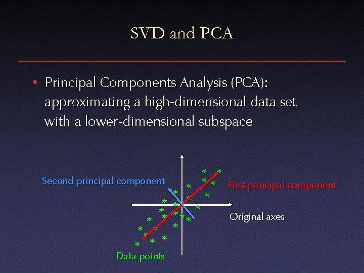
Principal Components Analaysis • Principal Components Analysis (PCA): approximating a high-dimensional data set with a lower-dimensional subspace Second principal component * ** * * Data points * * * First principal component * * *** Original axes *

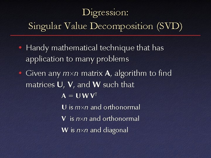
Digression: Singular Value Decomposition (SVD) • Handy mathematical technique that has application to many problems • Given any m n matrix A , algorithm to find matrices U, V , and W such that A = U W VT U is m n and orthonormal V is n n and orthonormal W is n n and diagonal

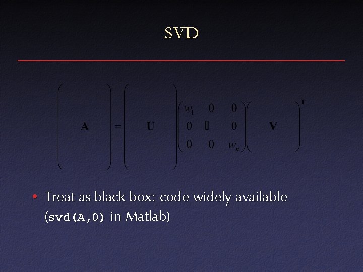
SVD • Treat as black box: code widely available (svd(A, 0) in Matlab)

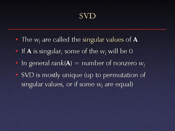
SVD • The wi are called the singular values of A • If A is singular, some of the wi will be 0 • In general rank (A ) = number of nonzero wi • SVD is mostly unique (up to permutation of singular values, or if some wi are equal)

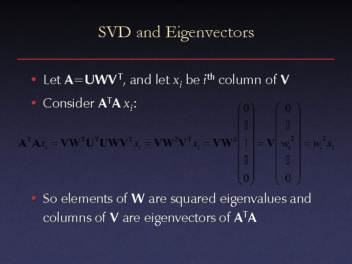
SVD and Eigenvectors • Let A =UWV T, and let x i be ith column of V • Consider A TA x i: • So elements of W are squared eigenvalues and columns of V are eigenvectors of A TA

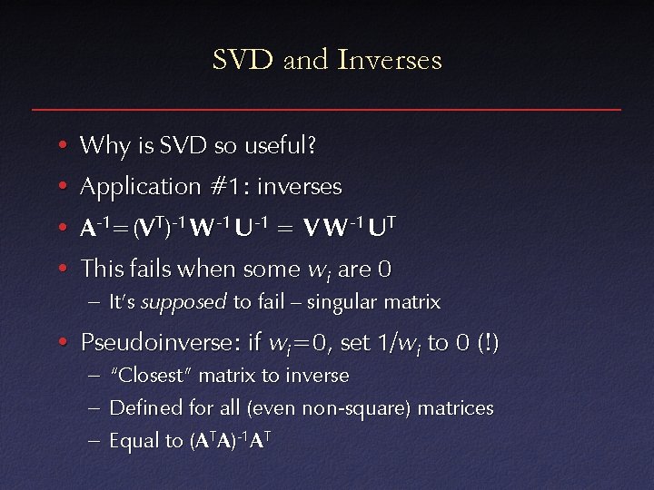
SVD and Inverses • Why is SVD so useful? • Application #1: inverses • A -1=(V T)-1 W -1 U-1 = V W -1 UT • This fails when some wi are 0 – It’s supposed to fail – singular matrix • Pseudoinverse: if wi=0, set 1/wi to 0 (!) – “Closest” matrix to inverse – Defined for all (even non-square) matrices – Equal to (ATA)-1 AT

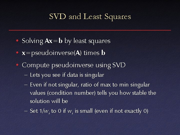
SVD and Least Squares • Solving Ax =b by least squares • x=pseudoinverse(A ) times b • Compute pseudoinverse using SVD – Lets you see if data is singular – Even if not singular, ratio of max to min singular values (condition number) tells you how stable the solution will be – Set 1/wi to 0 if wi is small (even if not exactly 0)

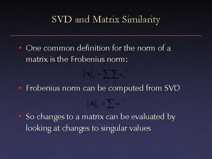
SVD and Matrix Similarity • One common definition for the norm of a matrix is the Frobenius norm: • Frobenius norm can be computed from SVD • So changes to a matrix can be evaluated by looking at changes to singular values

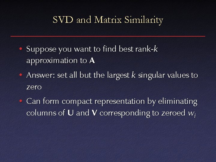
SVD and Matrix Similarity • Suppose you want to find best rank-k approximation to A • Answer: set all but the largest k singular values to zero • Can form compact representation by eliminating columns of U and V corresponding to zeroed wi

SVD and Orthogonalization • The matrix U is the “closest” orthonormal matrix to A • Yet another useful application of the matrixapproximation properties of SVD • Much more stable numerically than Graham-Schmidt orthogonalization • Find rotation given general affine matrix

SVD and PCA • Principal Components Analysis (PCA): approximating a high-dimensional data set with a lower-dimensional subspace Second principal component * ** * * Data points * * * First principal component * * *** Original axes *

SVD and PCA • Data matrix with points as rows, take SVD – Subtract out mean (“whitening”) • Columns of V k are principal components • Value of wi gives importance of each component

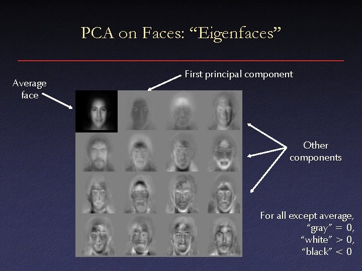
PCA on Faces: “Eigenfaces” Average face First principal component Other components For all except average, “gray” = 0, “white” > 0, “black” < 0

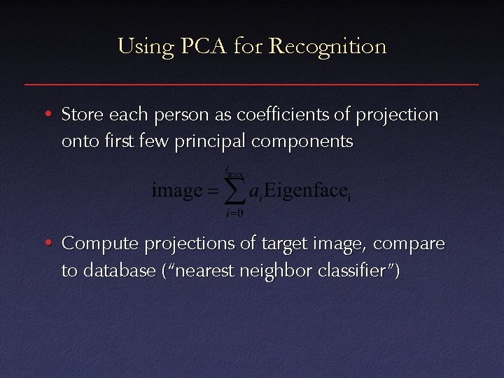
Using PCA for Recognition • Store each person as coefficients of projection onto first few principal components • Compute projections of target image, compare to database (“nearest neighbor classifier”)