Recent Development of the JMA Global Spectral Model

Recent Development of the JMA Global Spectral Model Masayuki Nakagawa JMA/NPD, visiting NCEP/EMC Nov. 10, 2009

Outline of the Presentation • Overview of JMA • Operational NWP models at JMA • Recent development in global NWP – Global Spectral Model – Ensemble Prediction System • Future plan

Overview of JMA

Structure of Central Government of Japan JMA is placed as an extra-ministerial bureau of the Ministry of Land, Infrastructure, Transport and Tourism. Total staff: ~5700 Budget: approx. $700 million/yr

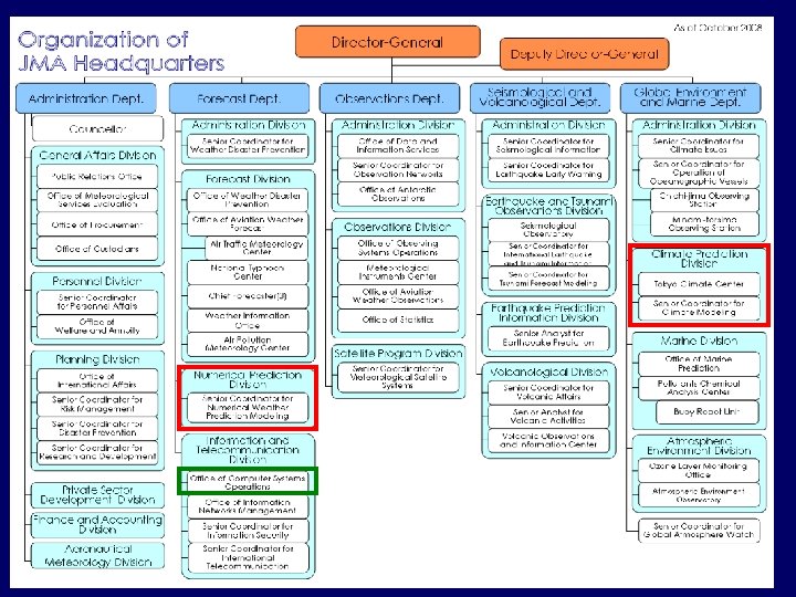
Organizational Structure of JMA

Observation Networks (1) • Surface observations – 156 manned weather stations – 1337 automatic weather stations • Radars – 11 Doppler radars – 9 conventional radars

Observation Networks (2) • Upper air observations – 16 radiosonde stations – 31 wind profilers • Satellite observations – Geostationary meteorological satellite (MTSAT -1 R) picture from the WMO homepage (modified)

Organization of NPD Numerical Prediction Division (74) – Administration Section (5) – Programming Section (11) • Management of NWP system • Development of data decoding system – Numerical Analysis and Modeling Section (46) • • • Development of NWP models and analysis systems Chief (1) Global Modeling Group (17) Mesoscale Modeling Group (13)　 Observation Group (15) – Application Section (12) • Development of applications (guidance, graphics, …)

Operational NWP models at JMA

Operational NWP Models at JMA (1) • Global model • Horizontal Resolution: 20 km • Updates: 4 times a day • Forecast domain: Global • Mesoscale model • Horizontal Resolution: 5 km • Updates: 8 times a day • Forecast domain: Japan and its surrounding areas

Operational NWP Models at JMA (2) One-week Ensemble Model One-month Ensemble Model Three-month Ensemble Model Warm/Cold season Ensemble Model One week forecast One month forecast Three month forecast Warm/Cold season outlook 1. 125 deg. / 320 x 160 (TL 159) 1. 875 deg. / 192 x 96 (TL 95) Global Model (GSM) Mesoscale Model (MSM) Typhoon Ensemble Model Short- and mediumrange forecast Warnings and very short- range forecast Typhoon forecast Forecast domain Global Japan and its surrounding areas Global Grid size/ Number of grids 0. 1875 deg. / 1920 x 960 (TL 959) 5 km/ 721 x 577 0. 5625 deg. / 640 x 320 (TL 319) Vertical levels/ Top 60 / 0. 1 h. Pa 50 / 21800 m 60 / 0. 1 h. Pa Purposes Forecast hours (initial time) 84 hours (00, 06, 18 UTC), 216 hours (12 UTC) 15 hours (00, 06, 12, 18 UTC), 33 hours (03, 09, 15, 21 UTC) 132 hours (00, 06, 12, 18 UTC) 11 members Analysis 4 D-Var Global analysis with ensemble perturbations 9 days (12 UTC) 51 members 34 days (12 UTC; Wed. & Thu. ) 25 members x 2 120 days (12 UTC; once a month) 31 members 150 -210 days (12 UTC; 5 times a year (Feb. , Mar. , Apr. , Sep. & Oct. ) 31 members

Framework of GSM • Resolution TL 959, reduced Gaussian grid 0. 1875 deg. / 1920 (equator) – 6 deg. / 60 (closest to pole) x 960, roughly 20 km 60 unevenly spaced sigma-p hybrid levels (surface to 0. 1 h. Pa) • Dynamics 2 -time level, semi-Lagrangian time integration Time step = 600 sec • Cumulus Prognostic Arakawa-Shubert • Cloud Prognostic cloud water • PBL Mellor and Yamada level II • Radiation(L) k-distribution method and table look-up method • Radiation(S) Lacis and Hansen (1974) • Gravity wave o(1 -10 km), o(100 km) • Land Si. B • Assimilation 4 D-Var

Operational Global Objective Analysis Cut-off time 2 h 20 m for early run analyses at 00, 06, 12 and 18 UTC, 11 h 35 m for cycle run analyses at 00 and 12 UTC, 5 h 35 m for cycle run analyses at 06 and 18 UTC Initial Guess 6 -hour forecast by GSM Grid form, resolution and number of grids Reduced Gaussian grid, 0. 1875 degree, 1920 x 960 for outer model Standard Gaussian grid, 0. 75 degree, 480 x 240 for inner model Levels 60 forecast model levels up to 0. 1 h. Pa + surface Analysis variables Surface pressure, temperature, winds and specific humidity Methodology Four-dimensional variational (4 D-Var) scheme on model levels Data Used SYNOP, SHIP, BUOY, TEMP, PILOT, wind profiler, AIREP, SATEM, ATOVS, SATOB, surface wind data from scatterometer on the Quik. SCAT satellite and MODIS wind data from Terra and Aqua; Typhoon bogussing applied for analysis Initialization Non-linear normal mode initialization and a vertical mode initialization for inner model Early Analysis: Analysis for weather forecast. The data cut off time is very short. Cycle Analysis: Analysis for keeping quality of global data assimilation system. This analysis is done after much observation data are received.

Roles of GSM • Basic information for a short- and medium-range, one week, one month and seasonal forecasts • Basic information for typhoon track and intensity forecasts • Assist of aviation and ship routing forecasts • Provision of lateral boundary condition for Mesoscale Model • Input data for ocean wave model • Input data for ocean data assimilation • Wind information for input of chemical transport model

Recent development in global NWP - GSM -

60 km FY 2004 GSM(T 213) 10 km GSM(TL 319) RSM 20 km Extend Forecast Time (NH)MSM Objective Analysis for 5 km FY 2003 GSM RSM MSM FY 2010 GSM(TL 959) (NH)MSM FY 2009 Ocean mixing layer model FY 2003 Major Forecast Models in JMA FY 2005 FY 2006 FY 2007 FY 2008 Reduced Gaussian grid Horizontal Resolution JMA/NWP – Update & Plan FY 2004 3 DVAR (T 106) Data Assimilation Systems FY 2005 FY 2006 FY 2007 FY 2008 4 DVAR (T 106) (T 63) 4 DVAR(40 km) FY 2009 FY 2010 4 DVAR (T 159) (TL 319) : RSM operation was finished 4 DVAR(20 km) (NH)4 DVAR(10 km) HPC System Upgrade * Japanese Fiscal Year : Start from April and End in March

Upgrade of GSM in Nov. 2007 previous Forecast time Horizontal resolution Vertical resolution Time integration orography/ mask Sea surface temperature Sea ice concentration Snow depth current 36（06, 18）/ 90（00）/ 216（12） 84（00, 06, 18）/ 216 hours（12 UTC） Approximately 60 km（TL 319） Approximately 20 km（TL 959） 40 layers（highest 0. 4 h. Pa） 60 layers（highest 0. 1 h. Pa） 3 -time level（Δt=900 sec） 2 -time level（Δt=600 sec） Equivalent to 60 km resolution Equivalent to 20 km resolution Daily analysis (1 degree resolution) Daily analysis (0. 25 degree resolution) Climatology (1 degree resolution) Daily analysis (0. 25 degree resolution) Daily analysis (1 degree resolution) 6 hourly analysis (higher resolution over Japan area)

Simulated Infrared Image 20 km-GSM TL 1023 L 40 2002. 7. 9. 00 Z FT=24 60 km-GSM T 213 L 40 2002. 7. 9. 00 Z FT=24 GMS-5 observation 00 UTC Jul. 10 2002

Orography of Operational Models at JMA GSM TL 959 (20 km) MSM (5 km) Orographic effects are better captured by higher resolution models. The surface parameters such as temperatures and winds, might be predicted more realistically by those models. GSM TL 319 (60 km)

Sigma-P Hybrid Vertical Level of GSM 0. 1 h. Pa about 65 km Stratosphere （25 layers） finer in lower atmosphere lowest level about 20 m Troposphere （35 layers）

Introduction of Reduced Gaussian Grid Miyamoto (2007) A reduced Gaussian grid was implemented in GSM as a new dynamical core in August 2008. On the standard Gaussian grid, the longitudinal interval between two grid points at the high latitudes is smaller than that at the low latitudes. Hence, it is redundant to use an equal number of grid points for all given latitudes in global model. The total number of gridpoints is reduced by about 30% in the reduced Gaussian grid, thus saving the computational throughput.

Moist Parameterization in GSM Ø Cumulus convection ü Arakawa-Schubert scheme (Arakawa and Shubert 1974; Moorthi and Suarez 1992; Randall and Pan 1993) ü Convection triggering mechanism proposed by Xie and Zhang (2000) (DCAPE) was introduced to improve the rainfall forecast Ø Clouds and large-scale precipitation ü Prognostic cloud water scheme (Sommeria and Deardorff 1977; Smith 1990) Ø Marine stratocumulus ü Stratocumulus scheme (diagnostic) (Slingo 1980, 1987; Kawai and Inoue 2006)

Convection Triggering Mechanism Xie and Zhang (2000) defined DCAPE (dynamic CAPE generation rate) as (T*, q*) are (T, q) plus the change due to the total large-scale advection over a time interval Δt (integration time step used in the model). They are equal to (T, q) just after the calculation of model dynamics. Xie and Zhang (2000) showed a strong relationship between deep convection and positive DCAPE. In TL 959 L 60 GSM, deep convection (cloud top < 700 h. Pa) is assumed to occur only when DCAPE> -1/300 (J/kg/s) , which corresponds to dynamic warming or moistening in the lower troposphere.

Precipitation (Typhoon) T 0610 TL 959 L 60 TL 319 L 40 Radar 6 hour accumulated precipitation valid at 12 UTC 18 August 2006. The initial time of the forecasts is 12 UTC 17 August 2006. The gray area in right panel indicate an absence of analysis. Typhoon T 0610 (WUKONG) was moving northward over Kyushu Island. Both models predicted its position well. TL 319 L 40 GSM could not predict the detailed distribution of precipitation and strong rainfall over land. TL 959 L 60 GSM simulated the distribution and intensity of precipitation better then TL 319 L 40 GSM, including orographic precipitation and heavy rainfall near the center of the typhoon.

RMSE and Bias of Typhoon Central Pressure 0 24 48 Forecast time (hour) 72 TYM: 24 -km resolution regional model covering a tropical cyclone and its surrounding areas. Its operation was terminated in November 2007. TL 319 L 40 GSM predicted weak typhoons compared to the best track analyzed by RSMC-Tokyo Typhoon Center because of its low horizontal resolution. TL 959 L 60 GSM predicted the typhoon intensity better then TL 319 L 40 GSM.

Precipitation Scores against Raingauge Observation (Aug. 2004) Bias score Threat score Threshold [mm/12 h] FT=36～ 48 hrs, 80 km grid average over Japan GSM tends to overestimate week precipitation areas and to underestimate strong precipitation areas in summer. : TL 959 L 60 : TL 319 L 40 : RSM (retired)

Precipitation Scores against Raingauge Observation (Aug. 2004) Bias score 0 12 [JST] Forecast hour [h] 80 km grid average over Japan Threshold: 1 mm/3 h : TL 959 L 60 : TL 319 L 40 : RSM (retired) The Introduction of convection triggering mechanism proposed by Xie and Zhang (2000) (DCAPE) reduced the tendency of GSM to overestimate weak precipitation areas especially from local noon to late afternoon.

Northern Hemisphere RMSE Aug. – Sep. 2004 TL 959 L 60： TL 319 L 40： Psea z 500 Dec. 2005 – Jan. 2006 Psea z 500 RMSE of Psea and z 500 decreased slightly in both summer and winter season. TL 959 L 60： TL 319 L 40：

Verification Score RMSE of 24, 48 and 72 hour forecasts by GSM for 500 h. Pa geopotential height against analysis in NH (20 N – 90 N). Curves: monthly means, horizontal lines: yearly means.

Pie chart showing the relative cost of various components for 84 hours forecast Resolution: TL 959 L 60 Disk access (20%) Computer: HITACHI SR 11000 70 nodes(140 MPIs) Real Time: 31 min 24 sec (fastest case: 29 min 39 sec) Calculation (44%) Communication (36%) After Miyamoto (2008)

Recent development in global NWP - EPS -

Upgrade of 1 W-EPS in Nov. 2007 previous Horizontal resolution Vertical resolution Time integration orography/ mask current Approximately 120 km（TL 159） Approximately 60 km（TL 319） 40 layers（highest 0. 4 h. Pa） 60 layers（highest 0. 1 h. Pa） 3 time level（Δt=1200 sec） 2 time level（Δt=1200 sec） Equivalent to 120 km resolution Equivalent to 60 km resolution Method to make initial perturbations Breeding of Growing Mode method Singular Vector method Perturbed area Northern hemisphere and tropical zone (20 S – 90 N) Ensemble size 51 members

Specification of Typhoon EPS (Feb. 2008) Purpose Improve both deterministic and probabilistic forecasts of tropical cyclone (TC) movement Forecast domain Global Grid size/ Number of grids 0. 5625 deg. / 640 x 320 (TL 319) Vertical levels/Top 60 / 0. 1 h. Pa Forecast hours 132 hours (00, 06, 12, 18 UTC) Runs when TCs of TS/STS/TY intensity exist in the responsibility area of RSMC Tokyo - Typhoon Center (0 N-60 N, 100 E-180 E) or are expected to move into the area within the next 24 hours Ensemble size 11 members Method to make initial perturbations Singular Vector (SV) method Linear combination of SVs targeted on both TCs (up to three TCs in one forecast event) and a mid-latitude region It is possible to obtain reliability of typhoon track forecast from the ensemble spread of typhoon track forecasts by Typhoon EPS. In addition, alternative track scenarios to an ensemble mean track are available.

Example of Typhoon Ensemble forecasts (1) T 0607 (MARIA) Typhoon Ensemble forecasts Forecast by GSM (11 members; blue line: control run) Analyzed track Possibility of recurvature of the typhoon is represented in Typhoon Ensemble forecasts. Ensemble spread is large, which indicates the reliability of the forecasts is relatively low.

Example of Typhoon Ensemble forecasts (2) T 0416 (CHABA) Typhoon Ensemble forecasts Forecast by GSM (11 members, blue line: control run) Analyzed track Ensemble spread is quite small, which indicates the reliability of the forecasts is relatively high.

Future plan (GSM)

Focus of NPD’s recent efforts Ø Model bias ü Temperature, moisture, … Ø Spin-up ü Precipitation, … Ø Land-sea contrast in precipitation Ø Precipitation over tropical eastern Pacific ü Global circulation Ø Formation of Typhoon Ø Size of Typhoon ü Maximum wind radius Ø Intensity of Typhoon ü Ocean mixing layer model

Future Resolution Upgrade Plan (next supercomputer system) • Deterministic forecast – TL 959 L 60 → TL 959 L 100 Upgrade model dynamics and physics Introduce new satellite data • Probabilistic forecast – 1 WEPS　TL 319 L 60 M 51 → TL 479 L 100 M 51 Improve representation of smaller scale phenomena Improve forecast skill of severe weather – TEPS　TL 319 L 60 M 11 → TL 479 L 80 M 25 Improve probabilistic forecast skill of tropical cyclone movement Improve forecast skill of severe weather associated with tropical cyclones

Thank you! Hare-run: JMA’s mascot Hare: Japanese word for “fine weather. ”

Replacement of JMA Supercomputer Previous System Mar 2001 -Feb 2006 Current System Mar 2005 - Mar 2006 - 50 nodes HITACHI SR 8000 E 1 -80 nodes 768 Gflops 80 nodes HITACHI SR 11000 J 1 -210 nodes 27. 5 Tflops

Early Analysis and Cycle Analysis Early Analysis: Analysis for weather forecast. The data cut off time is very short. Cycle Analysis: Analysis for keeping quality of global data assimilation system and for supplying the first guess to early analysis. This analysis is done after much observation data are received. Early Analysis Ea 00 in hurry to issue forecast 84 hour forecast Ea 06 Da 00 Cycle Analysis Da 18 Da 12 216 hour forecast 84 hour forecast Ea 18 Da 06 84 hour forecast The first guesses for Ea 06 and Ea 18 are supplied from Ea 00 and Ea 12, respectively. in hurry to issue forecast Ea 12 Early Analysis

Numerical/Dynamical Properties (1) • Horizontal representation – Spectral (spherical harmonic basis functions) with transformation to a reduced Gaussian grid for calculation of nonlinear quantities and most of the physics. • Horizontal resolution – Spectral triangular TL 959 (deterministic), TL 319 (EPS) • Vertical representation – Finite differences in sigma-pressure hybrid coordinates. • Vertical domain – Surface to 0. 1 h. Pa. • Vertical resolution – There are 60 unevenly spaced hybrid levels.

Numerical/Dynamical Properties (2) • Time integration scheme – A two-time level semi-implicit semi-Lagrangian scheme is used for the time integration. – A constant time step length 600 sec. is used for the deterministic (TL 959) model. • Equations of state – Primitive equations for dynamics in a spectral semi. Lagrangian framework are expressed in terms of wind components, temperature, specific humidity, cloud water and surface pressure. • Diffusion – A linear fourth-order horizontal diffusion is applied on the hybrid sigma-pressure surfaces in spectral space.

Physical Properties • • Cumulus Cloud PBL Radiation(L) Prognostic Arakawa-Shubert Prognostic cloud water Mellor and Yamada level II k-distribution method and table look-up method • Radiation(S) Lacis and Hansen (1974) • Gravity wave o(1 -10 km), o(100 km) • Land Si. B

Reduced Gaussian Grid (Aug. 2008) There a large number of redundant grid-points and insignificant wavenumber components in the standard Gaussian grid. The total number of gridpoints is reduced by about 30% in the reduced Gaussian grid. Latitude Reduced Gaussian grid Standard Gaussian grid After Miyamoto (2007) The number of longitudinal grid points … must be the multiples of the number of longitudinal sub-domains. must be the composite numbers of the radices of FFT kernels. Longitudinal grid interval (km) should be the multiple numbers of the longitudinal interval of the radiation process.

Convection and precipitation • deep convection - Arakawa and Schubert 1974 • conversion of cloud droplets to precipitation • moisture detrainment from top of the cumulus • re-evaporation of stratiform precipitation Short-wave radiation Long-wave radiation upward mass flux detrainment Water vapor condensation evaporation Cloud water Conversion from cloud droplets reevaporati on precipitation Cumulus convection entrainment convective downdraft compensative downdraft

Simple Biosphere model lowest level of the atmospheric model sensible heat canopy latent heat sw rad. grass lw rad. bare ground thin skin layer soil layer Snowmass is not treated explicitly and is regarded as an iced water on the grass or bare ground. Upper 5 cm snow is accounted in heat budget conductive heat (evaluated with force restore method)

Transition Steps Ø Algorithm development Ø Preliminary testing ü Low resolution (TL 319 L 60) forecast/assimilation experiment, summer and winter ü High resolution (TL 959 L 60) single forecast experiment (no assimilation) Ø Pre-Implementation testing ü High resolution (TL 959 L 60) forecast/assimilation experiment, at least summer and winter ü Systematic error, RMSE, anomaly correlation, typhoon track and intensity, precipitation, … Ø Implementation

Introduction of new convection triggering function to Arakawa. Schubert scheme

Moist parameterization in GSM Ø Cumulus convection ü Arakawa-Schubert scheme l Convection triggering function l Rainwater and cloud water budget Ø Clouds and large-scale precipitation ü Cloud water scheme Ø Marine stratocumulus ü Stratocumulus scheme

Convection triggering function (1) Radar observation GSM forecast GSM tends to predict convective precipitation too early with too wide areas in summer daytime. In order to improve the rainfall forecast, a new convection triggering mechanism is introduced. Xie and Zhang (2000) showed a strong relationship between deep convection and positive DCAPE (dynamic CAPE generation rate) which is determined by the large scale advective tendencies. 6 hour accumulated precipitation, 12 UTC 18 July 2005 initial, FT=18 (15 local time).

Convection triggering function (2) Xie and Zhang (2000) defined DCAPE (dynamic CAPE generation rate) as (T*, q*) are (T, q) plus the change due to the total largescale advection over a time interval Δt (integration time step used in the model). They are equal to (T, q) just after the calculation of model dynamics.

40 0. 1 10 0 1 Radar obs. GSM w/o DCAPE GSM with DCAPE 6 hour accumulated precipitation and DCAPE valid at 12 UTC 18 July 2005. Initial time of forecasts is 12 UTC 17 July 2005. Precipitating area is closely related to the area where DCAPE>0, which suggests the capability of DCAPE as the triggering function of deep convection. In TL 959 L 60 GSM, deep convection (cloud top < 700 h. Pa) is assumed to occur only when DCAPE> -1/300 (J/kg/s) , which corresponds to dynamic warming or moistening in the lower troposphere. The threshold value depends on horizontal resolution.

Case study (thunderstorm) GSM w/o DCAPE GSM with DCAPE Radar obs. 6 hour accumulated precipitation valid at 12 UTC 9 August 2004. Initial time of forecasts is 12 UTC 8 August 2004. GSM without DCAPE predicts too weak and wide precipitation. GSM with DCAPE simulates the areas and the intensity of thunderstorm better than that without DCAPE.

Case study (Typhoon T 0416) GSM w/o DCAPE GSM with DCAPE Radar obs. T 0416 6 hour accumulated precipitation valid at 00 UTC 30 August 2004. Initial time of forecasts is 12 UTC 28 August 2004. GSM without DCAPE predicts too weak precipitation. GSM with DCAPE simulates the areas and the intensity of heavy precipitation better than that without DCAPE.

Statistics Bias and equitable threat scores of 3 hour accumulated precipitation forecasts against raingauge observation over Japan for August 2004. Horizontal axis: forecast time. Bias score for weak precipitation (1 mm/3 hour) of GSM without DCAPE (blue) is larger than 1 and shows strong diurnal variation. The variation is reduced substantially in GSM with DCAPE (red), though the bias is still large.

Summary Ø The convection triggering mechanism proposed by Xie and Zhang (2000) (DCAPE) was introduced to the A-S scheme to improve the rainfall forecast. Ø GSM with DCAPE simulated the area and the intensity of heavy precipitation associated with thunderstorm and typhoon better than GSM without DCAPE. Ø The tendency of GSM to overestimate weak precipitation areas especially from local noon to late afternoon is also reduced. Ø DCAPE is implemented to the operational GSM in November 2007.