Recapitulate The Physical interpretation of wave function Time

Recapitulate The Physical interpretation of wave function. Time independent Schrödinger Equation. Energy quantization in particle in a box case.

Example: Particle in a Rigid Box x=0 x=L

For x<0 and x>L For 0<x<L The general solution of this equation is

Boundary Conditions The wave function must be continuous. This implies that This gives

This is possible only when

Notes We had two unknowns with three equation (including normalization condition). The additional equation quantized the energy levels. The values of n can only be positive and non-zero. The lowest energy is non-zero (zeropoint energy).

The lowest energy corresponding to n=1 for an electron in a box of 1Å comes out to be 37. 6 e. V. For a marble of 0. 01 kg in 0. 1 m box it is 5. 488 x 10 -64 J. It would take 1020 years to move one mm.

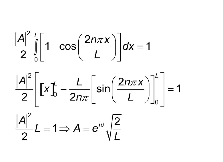
Normalization We must have Realizing that k can take only discrete values, we replace k.

We take the phase angle to be zero. This gives us

Wave function and Probability x=0 x=L What do you expect classically?

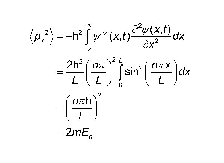
Expected Values

The last step can be obtained by integrating by parts.

Verify last step after integrating by

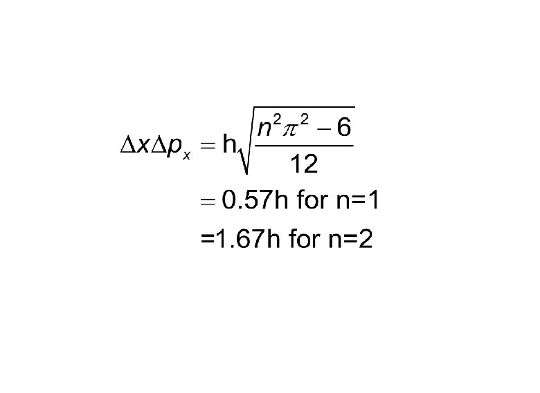
Uncertainties

Orthonormality of Wave function We can show that Here the Kronecker-Delta function is defined as follows.

Proof

Expansion Any function f(x) that is defined between x=0 and x=L and zero everywhere else can be expressed as follows.

The above can be easily visualized using the orthonormality property of the wave function

The interpretation of the coefficients We had earlier said that the following is a valid wave function at time t=0.

We now give the physical interpretation of the coefficients. Starting with normalized ψ(x, 0), implying is equal to the probability of finding the particle in nth state.

Example Following are the two normalized wave function corresponding to n=1 and n=4 states.

Following wave function is not a normalized wave function. The above can be seen by evaluating

Also, we can see that The normalized wave function would thus be

The physical interpretation implies imagining a large number of boxes where the wavefunction of the particle is given by above. If a measurement of energy is done, in half of them we shall find the particle to be in n=1 and in another half in n=4 state.

Question 1: Is the following wave function a normalized one?

We can write the above as follows. In this case in 20% of the boxes will give an energy corresponding to n=1 and 80% corresponding to n=4.

Question 2: What would be the expected value of energy in such a case?

Question 3: If no measurement was done what would be the wave function at a time t. We can check that this would not be a stationary state and the probability of finding the particle at a location would be a function of time.

Question 4: If a measurement is done in one of the boxes at t=0 and the energy is found to be E 4, what would be the wave function at a later time t. The wave function now collapses and the time dependence would be given by.

Question 5: What would the measurement of energy yield on this box at a later time? The particle is now in stationary state. Hence the measurement would lead to E 4.

SOME POSTULATES OF QM

1. System Description and Time Evolution A particle under a potential V(x) is described by a wave function ψ(x), which contains the information about all the physical properties of the particle. The time evolution of ψ(x) is governed by the time dependent Schrödinger Equation.

The wave function ψ(x) is single valued, finite and a continuous function of x. The position derivative is also continuous , unless V(x) shows infinite jump.

Compare From Krane (Modern Physics): When an object moves across the boundary between two regions in which it is subjected to different [forces, potential energies], the basic behavior of the object is found by solving [Newton’s second law, the Schrodinger equation].

The [position, wave function] of the object is always continuous across the boundary, and the [velocity, derivative dψ/dx] is also continuous as long as the [force, change in potential energy] remains finite.

2. Operators Each dynamical variable that relates to the motion of the particle can be represented by an operator, satisfying certain criteria. The only possible result of a measurement of the dynamical variable represented by an operator is one or the other Eigen values of the operator.

The Eigen values are real numbers for the operators representing dynamical variables.

Hamiltonian Operator It is defined as follows Eigen Value Equation of Hamiltonian Operator is thus

Replacing by their operators we get

3. Completeness The Eigen States of an operator representing a dynamical variable are complete. Any admissible wave function can always be expressed in the following way in terms of Eigen functions of any operator.

These Eigen functions form the basis. We had discussed this aspect in detail with Eigen function of the Hamiltonian operator.

4. Probability The probability that an Eigen value gn would be observed as a result of measurement is proportional to the square of the magnitude of the coefficient cn in the expansion of ψ. The proportionality become equality if we have normalized wave function.

5. Collapse of Wave function If the measurement gives a particular value of Eigen value gn, the wave function discontinuously collapses to.