Recap Mining association rules from large datasets Recap

Recap: Mining association rules from large datasets

Recap • Task 1: Methods for finding all frequent itemsets efficiently • Task 2: Methods for finding association rules efficiently

Recap • Frequent itemsets (measure: support) • Apriori principle • Apriori algorithm for finding frequent itemsets – Prunes really well in practice – Makes multiple passes over the dataset

Making a single pass over the data: the Apriori. Tid algorithm • The database is not used for counting support after the 1 st pass! • Instead information in data structure Ck’ is used for counting support in every step • Ck’ is generated from Ck-1’ • For small values of k, storage requirements for data structures could be larger than the database! • For large values of k, storage requirements can be very small

Lecture outline • Task 1: Methods for finding all frequent itemsets efficiently • Task 2: Methods for finding association rules efficiently

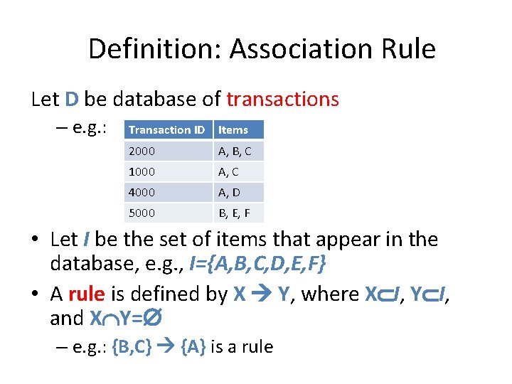
Definition: Association Rule Let D be database of transactions – e. g. : Transaction ID Items 2000 A, B, C 1000 A, C 4000 A, D 5000 B, E, F • Let I be the set of items that appear in the database, e. g. , I={A, B, C, D, E, F} • A rule is defined by X Y, where X I, Y I, and X Y= – e. g. : {B, C} {A} is a rule

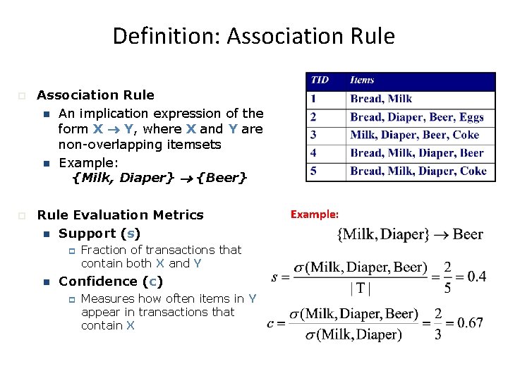
Definition: Association Rule An implication expression of the form X Y, where X and Y are non-overlapping itemsets Example: {Milk, Diaper} {Beer} Rule Evaluation Metrics Support (s) Fraction of transactions that contain both X and Y Confidence (c) Measures how often items in Y appear in transactions that contain X Example:

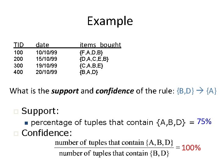
Example TID date items_bought 100 200 300 400 10/10/99 15/10/99 19/10/99 20/10/99 {F, A, D, B} {D, A, C, E, B} {C, A, B, E} {B, A, D} What is the support and confidence of the rule: {B, D} {A} Support: percentage of tuples that contain {A, B, D} = 75% Confidence: 100%

Association-rule mining task • Given a set of transactions D, the goal of association rule mining is to find all rules having – support ≥ minsup threshold – confidence ≥ minconf threshold

Brute-force algorithm for association-rule mining • List all possible association rules • Compute the support and confidence for each rule • Prune rules that fail the minsup and minconf thresholds • Computationally prohibitive!

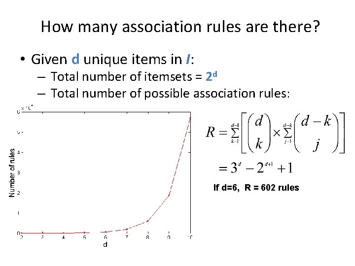
How many association rules are there? • Given d unique items in I: – Total number of itemsets = 2 d – Total number of possible association rules: If d=6, R = 602 rules

Mining Association Rules • Two-step approach: – Frequent Itemset Generation – Generate all itemsets whose support minsup – Rule Generation – Generate high confidence rules from each frequent itemset, where each rule is a binary partition of a frequent itemset

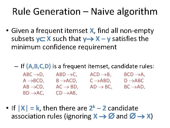
Rule Generation – Naive algorithm • Given a frequent itemset X, find all non-empty subsets y X such that y X – y satisfies the minimum confidence requirement – If {A, B, C, D} is a frequent itemset, candidate rules: ABC D, A BCD, AB CD, BD AC, ABD C, B ACD, AC BD, CD AB, ACD B, C ABD, AD BC, BCD A, D ABC BC AD, • If |X| = k, then there are 2 k – 2 candidate association rules (ignoring X and X)

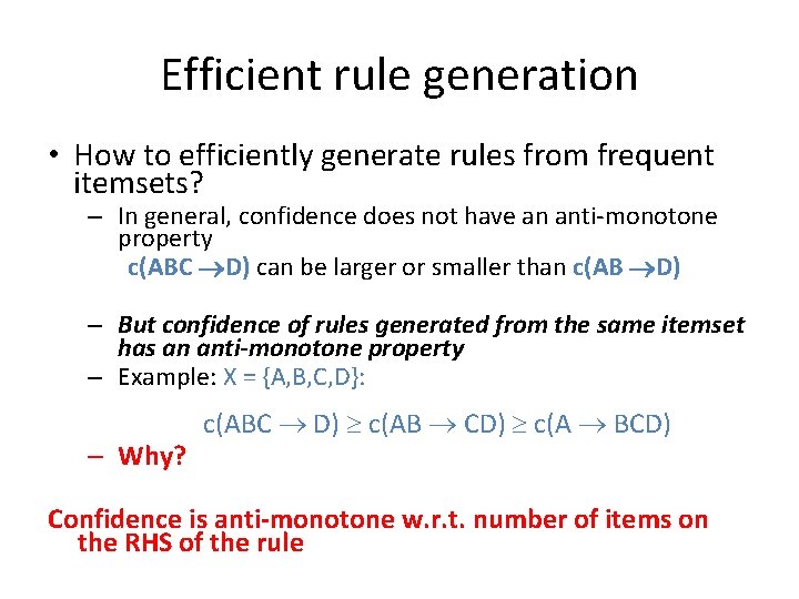
Efficient rule generation • How to efficiently generate rules from frequent itemsets? – In general, confidence does not have an anti-monotone property c(ABC D) can be larger or smaller than c(AB D) – But confidence of rules generated from the same itemset has an anti-monotone property – Example: X = {A, B, C, D}: – Why? c(ABC D) c(AB CD) c(A BCD) Confidence is anti-monotone w. r. t. number of items on the RHS of the rule

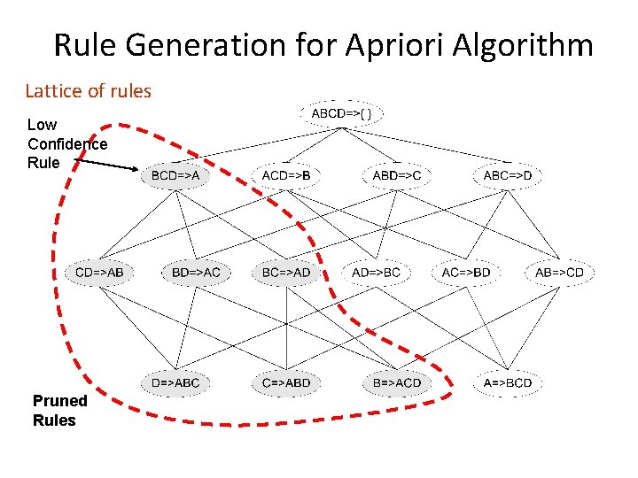
Rule Generation for Apriori Algorithm Lattice of rules Low Confidence Rule Pruned Rules

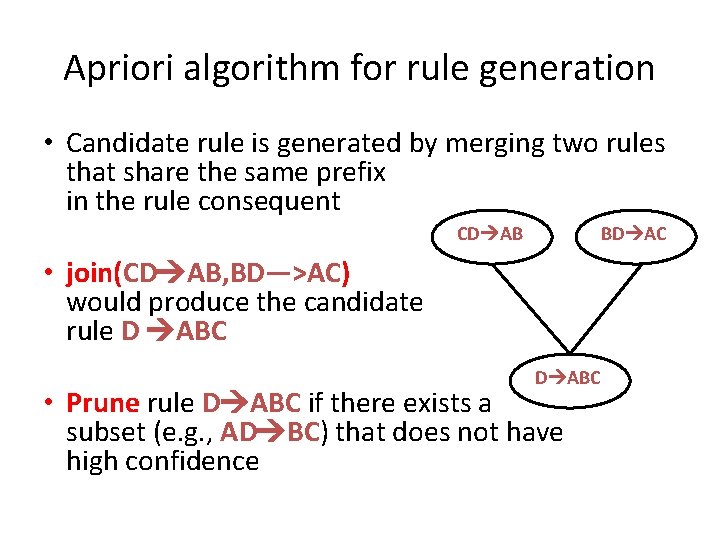
Apriori algorithm for rule generation • Candidate rule is generated by merging two rules that share the same prefix in the rule consequent CD AB BD AC • join(CD AB, BD—>AC) would produce the candidate rule D ABC • Prune rule D ABC if there exists a subset (e. g. , AD BC) that does not have high confidence

Reducing the collection of itemsets: alternative representations and combinatorial problems

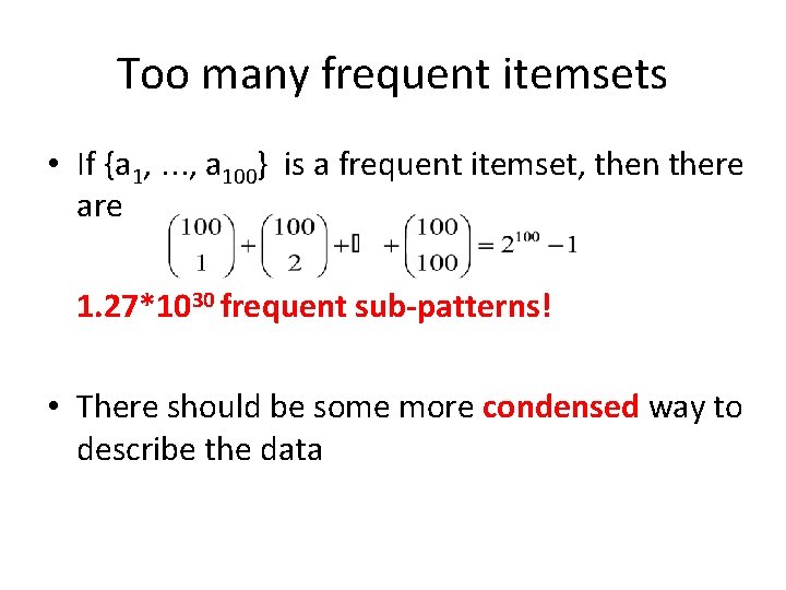
Too many frequent itemsets • If {a 1, …, a 100} is a frequent itemset, then there are 1. 27*1030 frequent sub-patterns! • There should be some more condensed way to describe the data

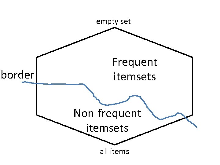
Frequent itemsets maybe too many to be helpful • If there are many and large frequent itemsets enumerating all of them is costly. • We may be interested in finding the boundary frequent patterns. • Question: Is there a good definition of such boundary?

empty set border Frequent itemsets Non-frequent itemsets all items

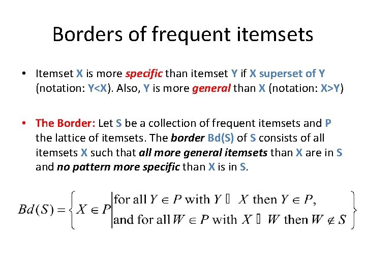
Borders of frequent itemsets • Itemset X is more specific than itemset Y if X superset of Y (notation: Y<X). Also, Y is more general than X (notation: X>Y) • The Border: Let S be a collection of frequent itemsets and P the lattice of itemsets. The border Bd(S) of S consists of all itemsets X such that all more general itemsets than X are in S and no pattern more specific than X is in S.

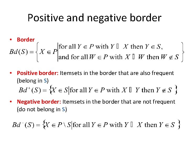
Positive and negative border • Border • Positive border: Itemsets in the border that are also frequent (belong in S) • Negative border: Itemsets in the border that are not frequent (do not belong in S)

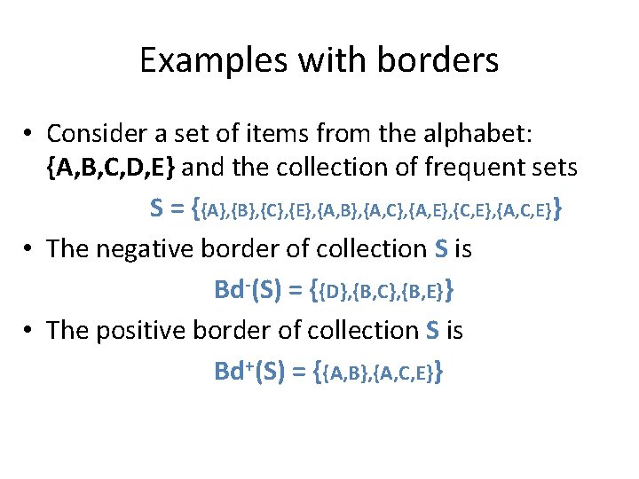
Examples with borders • Consider a set of items from the alphabet: {A, B, C, D, E} and the collection of frequent sets S = {{A}, {B}, {C}, {E}, {A, B}, {A, C}, {A, E}, {C, E}, {A, C, E}} • The negative border of collection S is Bd-(S) = {{D}, {B, C}, {B, E}} • The positive border of collection S is Bd+(S) = {{A, B}, {A, C, E}}

Descriptive power of the borders • Claim: A collection of frequent sets S can be fully described using only the positive border (Bd+(S)) or only the negative border (Bd-(S)).

Maximal patterns Frequent patterns without proper frequent super pattern

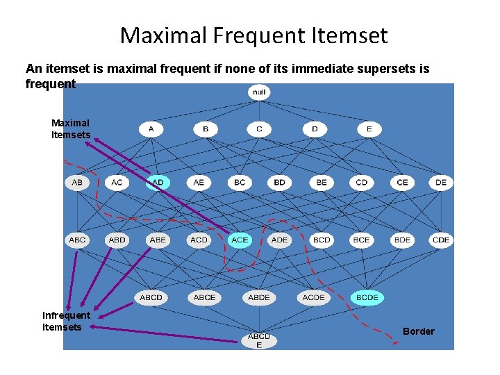
Maximal Frequent Itemset An itemset is maximal frequent if none of its immediate supersets is frequent Maximal Itemsets Infrequent Itemsets Border

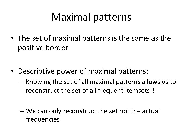
Maximal patterns • The set of maximal patterns is the same as the positive border • Descriptive power of maximal patterns: – Knowing the set of all maximal patterns allows us to reconstruct the set of all frequent itemsets!! – We can only reconstruct the set not the actual frequencies

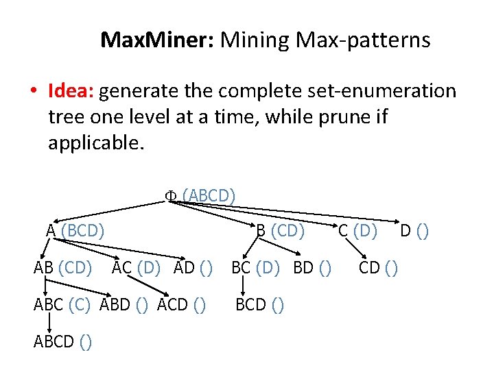
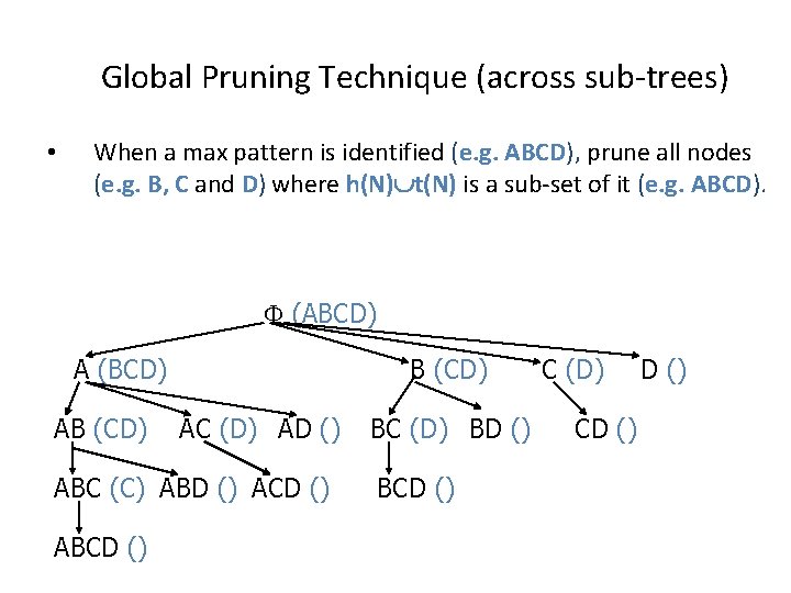
Max. Miner: Mining Max-patterns • Idea: generate the complete set-enumeration tree one level at a time, while prune if applicable. (ABCD) A (BCD) AB (CD) AC (D) AD () ABC (C) ABD () ACD () ABCD () BC (D) BD () BCD () C (D) CD ()

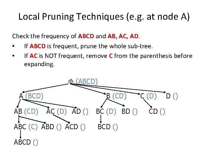
Local Pruning Techniques (e. g. at node A) Check the frequency of ABCD and AB, AC, AD. • If ABCD is frequent, prune the whole sub-tree. • If AC is NOT frequent, remove C from the parenthesis before expanding. (ABCD) A (BCD) AB (CD) AC (D) AD () ABC (C) ABD () ACD () ABCD () BC (D) BD () BCD () C (D) CD ()

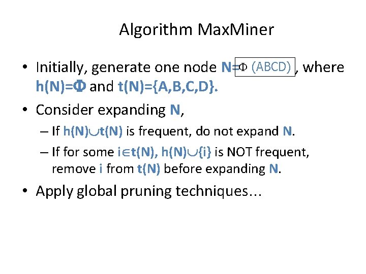
Algorithm Max. Miner • Initially, generate one node N= (ABCD) , where h(N)= and t(N)={A, B, C, D}. • Consider expanding N, – If h(N) t(N) is frequent, do not expand N. – If for some i t(N), h(N) {i} is NOT frequent, remove i from t(N) before expanding N. • Apply global pruning techniques…

Global Pruning Technique (across sub-trees) • When a max pattern is identified (e. g. ABCD), prune all nodes (e. g. B, C and D) where h(N) t(N) is a sub-set of it (e. g. ABCD). (ABCD) A (BCD) AB (CD) AC (D) AD () ABC (C) ABD () ACD () ABCD () BC (D) BD () BCD () C (D) CD ()

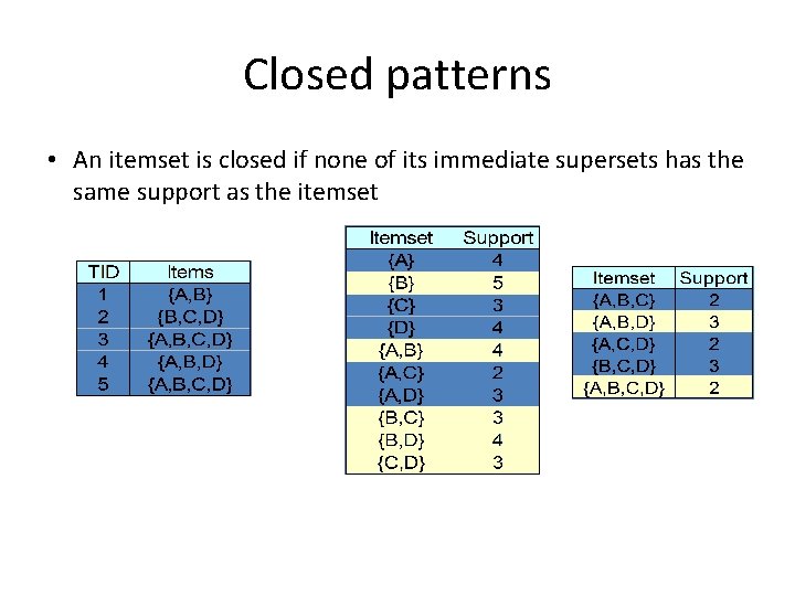
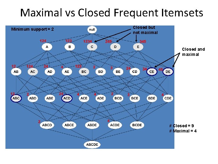
Closed patterns • An itemset is closed if none of its immediate supersets has the same support as the itemset

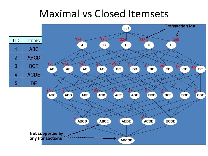
Maximal vs Closed Itemsets Transaction Ids Not supported by any transactions

Maximal vs Closed Frequent Itemsets Minimum support = 2 Closed but not maximal Closed and maximal # Closed = 9 # Maximal = 4

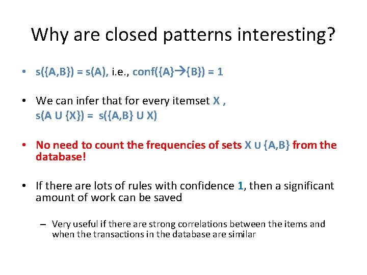
Why are closed patterns interesting? • s({A, B}) = s(A), i. e. , conf({A} {B}) = 1 • We can infer that for every itemset X , s(A U {X}) = s({A, B} U X) • No need to count the frequencies of sets X U {A, B} from the database! • If there are lots of rules with confidence 1, then a significant amount of work can be saved – Very useful if there are strong correlations between the items and when the transactions in the database are similar

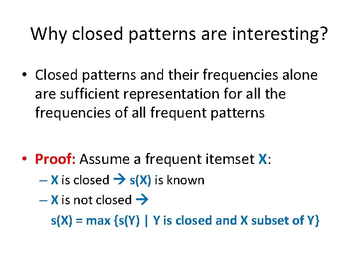
Why closed patterns are interesting? • Closed patterns and their frequencies alone are sufficient representation for all the frequencies of all frequent patterns • Proof: Assume a frequent itemset X: – X is closed s(X) is known – X is not closed s(X) = max {s(Y) | Y is closed and X subset of Y}

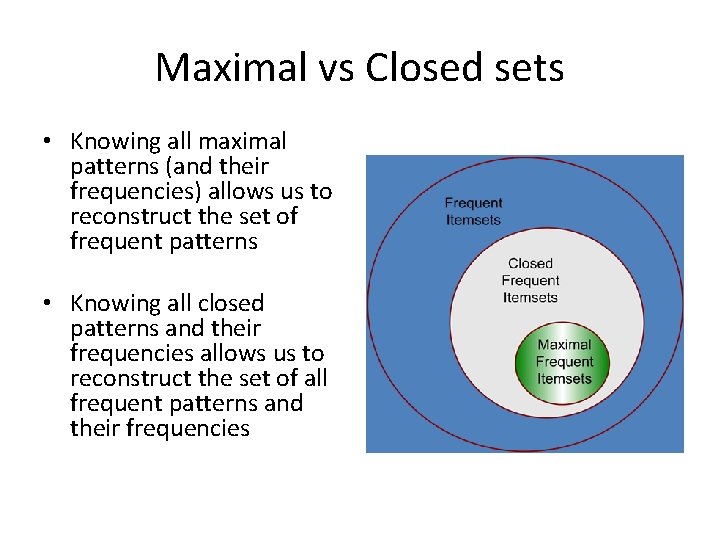
Maximal vs Closed sets • Knowing all maximal patterns (and their frequencies) allows us to reconstruct the set of frequent patterns • Knowing all closed patterns and their frequencies allows us to reconstruct the set of all frequent patterns and their frequencies

A more algorithmic approach to reducing the collection of frequent itemsets

Prototype problems: Covering problems • Setting: – Universe of N elements U = {U 1, …, UN} – A set of n sets S = {s 1, …, sn} – Find a collection C of sets in S (C subset of S) such that UcєCc contains many elements from U • Example: – U: set of documents in a collection – si: set of documents that contain term ti – Find a collection of terms that cover most of the documents

Prototype covering problems • Set cover problem: Find a small collection C of sets from S such that all elements in the universe U are covered by some set in C • Best collection problem: find a collection C of k sets from S such that the collection covers as many elements from the universe U as possible • Both problems are NP-hard • Simple approximation algorithms with provable properties are available and very useful in practice

Set-cover problem • Universe of N elements U = {U 1, …, UN} • A set of n sets S = {s 1, …, sn} such that Uisi =U • Question: Find the smallest number of sets from S to form collection C (C subset of S) such that UcєCc=U • The set-cover problem is NP-hard (what does this mean? )

Trivial algorithm • Try all subcollections of S • Select the smallest one that covers all the elements in U • The running time of the trivial algorithm is O(2|S||U|) • This is way too slow

Greedy algorithm for set cover • Select first the largest-cardinality set s from S • Remove the elements from U • Recompute the sizes of the remaining sets in S • Go back to the first step

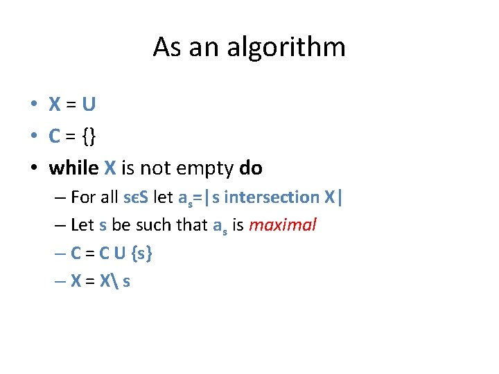
As an algorithm • X=U • C = {} • while X is not empty do – For all sєS let as=|s intersection X| – Let s be such that as is maximal – C = C U {s} – X = X s

How can this go wrong? • No global consideration of how good or bad a selected set is going to be

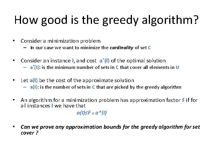
How good is the greedy algorithm? • Consider a minimization problem – In our case we want to minimize the cardinality of set C • Consider an instance I, and cost a*(I) of the optimal solution – a*(I): is the minimum number of sets in C that cover all elements in U • Let a(I) be the cost of the approximate solution – a(I): is the number of sets in C that are picked by the greedy algorithm • An algorithm for a minimization problem has approximation factor F if for all instances I we have that a(I)≤F x a*(I) • Can we prove any approximation bounds for the greedy algorithm for set cover ?

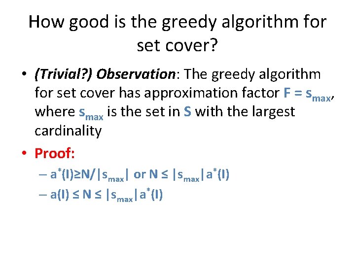
How good is the greedy algorithm for set cover? • (Trivial? ) Observation: The greedy algorithm for set cover has approximation factor F = smax, where smax is the set in S with the largest cardinality • Proof: – a*(I)≥N/|smax| or N ≤ |smax|a*(I) – a(I) ≤ N ≤ |smax|a*(I)

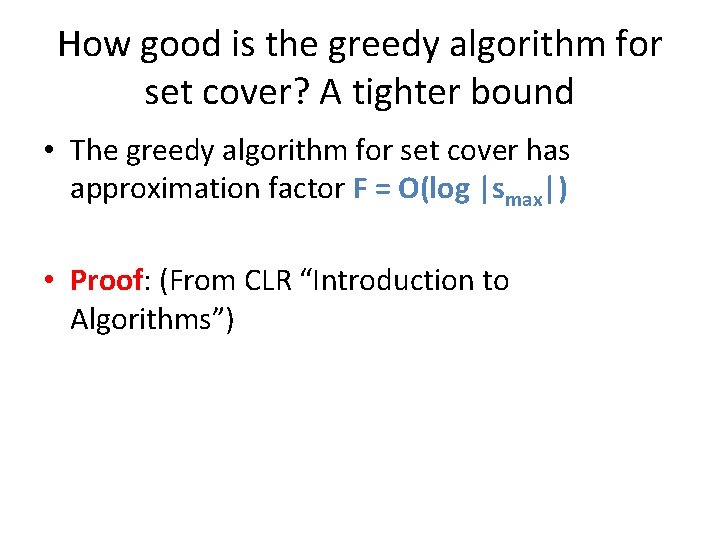
How good is the greedy algorithm for set cover? A tighter bound • The greedy algorithm for set cover has approximation factor F = O(log |smax|) • Proof: (From CLR “Introduction to Algorithms”)

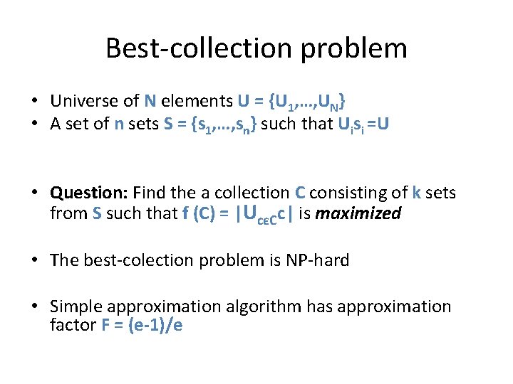
Best-collection problem • Universe of N elements U = {U 1, …, UN} • A set of n sets S = {s 1, …, sn} such that Uisi =U • Question: Find the a collection C consisting of k sets from S such that f (C) = |UcєCc| is maximized • The best-colection problem is NP-hard • Simple approximation algorithm has approximation factor F = (e-1)/e

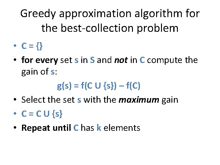
Greedy approximation algorithm for the best-collection problem • C = {} • for every set s in S and not in C compute the gain of s: g(s) = f(C U {s}) – f(C) • Select the set s with the maximum gain • C = C U {s} • Repeat until C has k elements

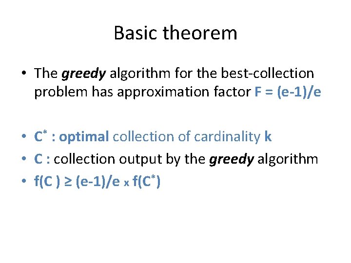
Basic theorem • The greedy algorithm for the best-collection problem has approximation factor F = (e-1)/e • C* : optimal collection of cardinality k • C : collection output by the greedy algorithm • f(C ) ≥ (e-1)/e x f(C*)

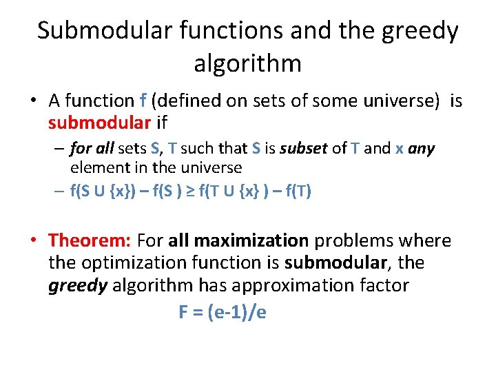
Submodular functions and the greedy algorithm • A function f (defined on sets of some universe) is submodular if – for all sets S, T such that S is subset of T and x any element in the universe – f(S U {x}) – f(S ) ≥ f(T U {x} ) – f(T) • Theorem: For all maximization problems where the optimization function is submodular, the greedy algorithm has approximation factor F = (e-1)/e

Again: Can you think of a more algorithmic approach to reducing the collection of frequent itemsets

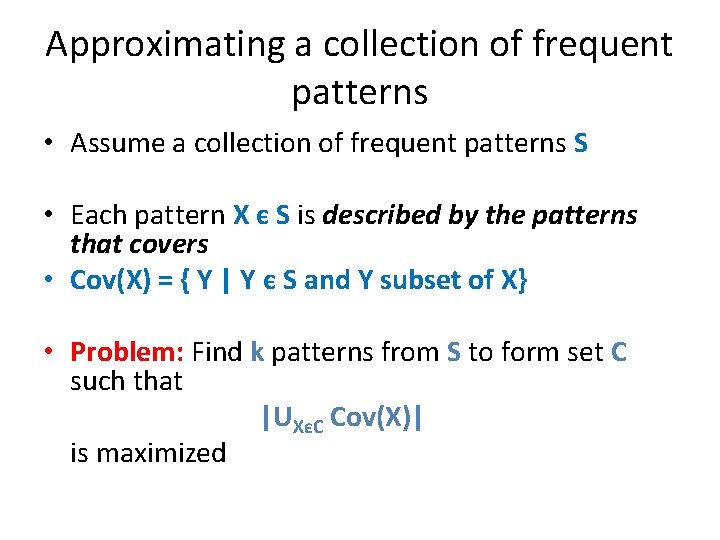
Approximating a collection of frequent patterns • Assume a collection of frequent patterns S • Each pattern X є S is described by the patterns that covers • Cov(X) = { Y | Y є S and Y subset of X} • Problem: Find k patterns from S to form set C such that |UXєC Cov(X)| is maximized

empty set border Frequent itemsets Non-frequent itemsets all items