Recap Light and Cameras Recap Frequency Domain Fourier

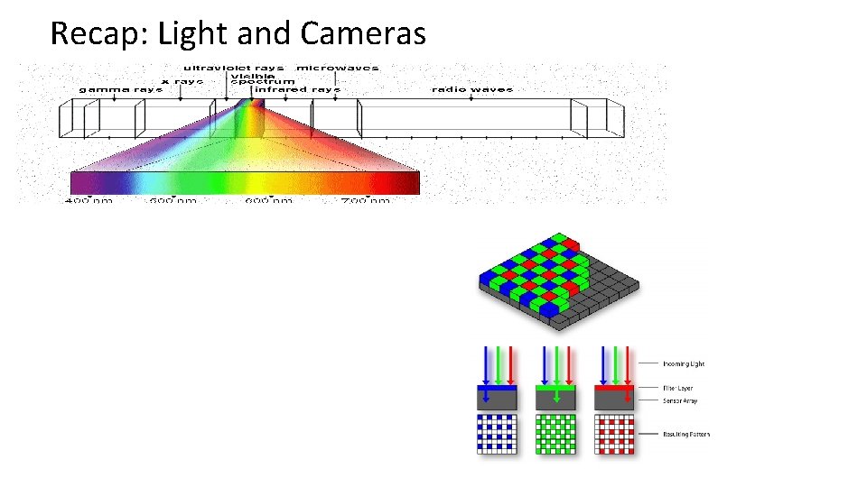
Recap: Light and Cameras

Recap: Frequency Domain

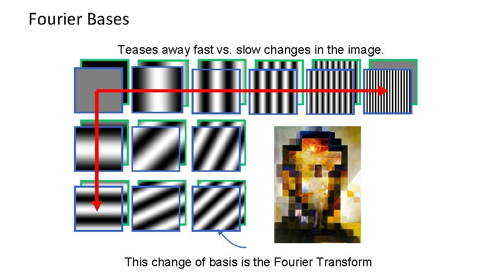
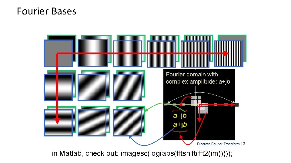
Fourier Bases Teases away fast vs. slow changes in the image. This change of basis is the Fourier Transform

Fourier Bases in Matlab, check out: imagesc(log(abs(fftshift(fft 2(im)))));

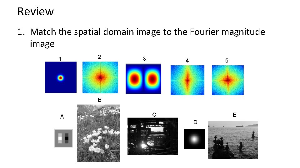
Review 1. Match the spatial domain image to the Fourier magnitude image 1 2 3 4 5 B A C E D

Interest Points and Corners Computer Vision James Hays Read Szeliski 7. 1. 1 and 7. 1. 2 Slides from Rick Szeliski, Svetlana Lazebnik, Derek Hoiem and Grauman&Leibe 2008 AAAI Tutorial

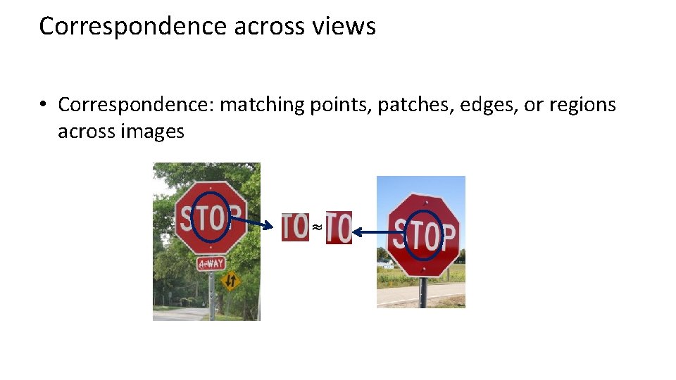
Correspondence across views • Correspondence: matching points, patches, edges, or regions across images ≈

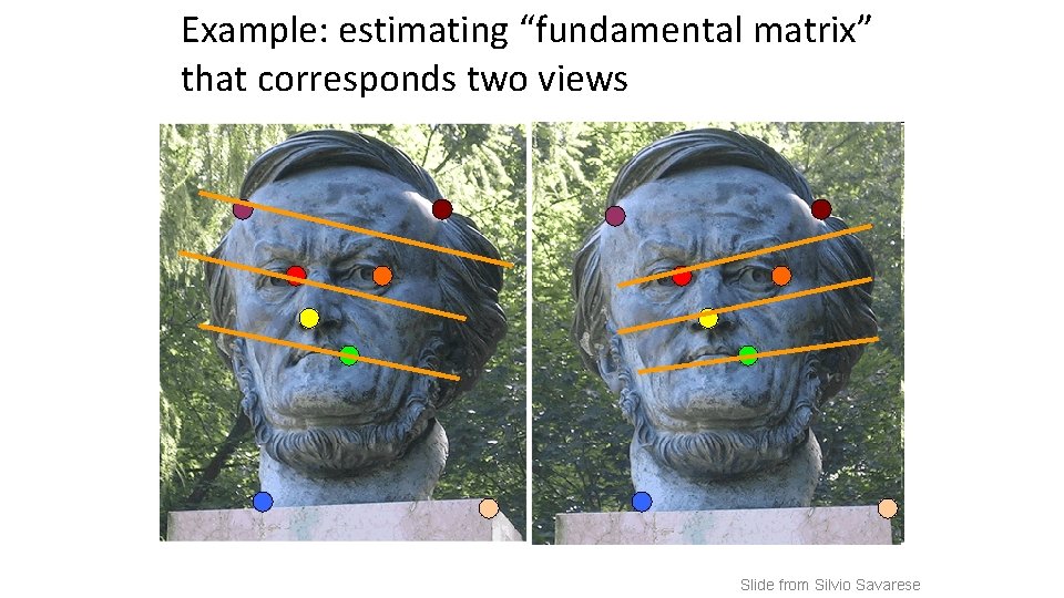
Example: estimating “fundamental matrix” that corresponds two views Slide from Silvio Savarese

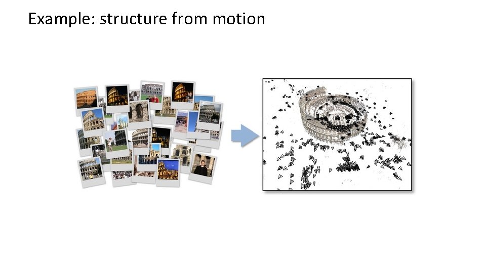
Example: structure from motion

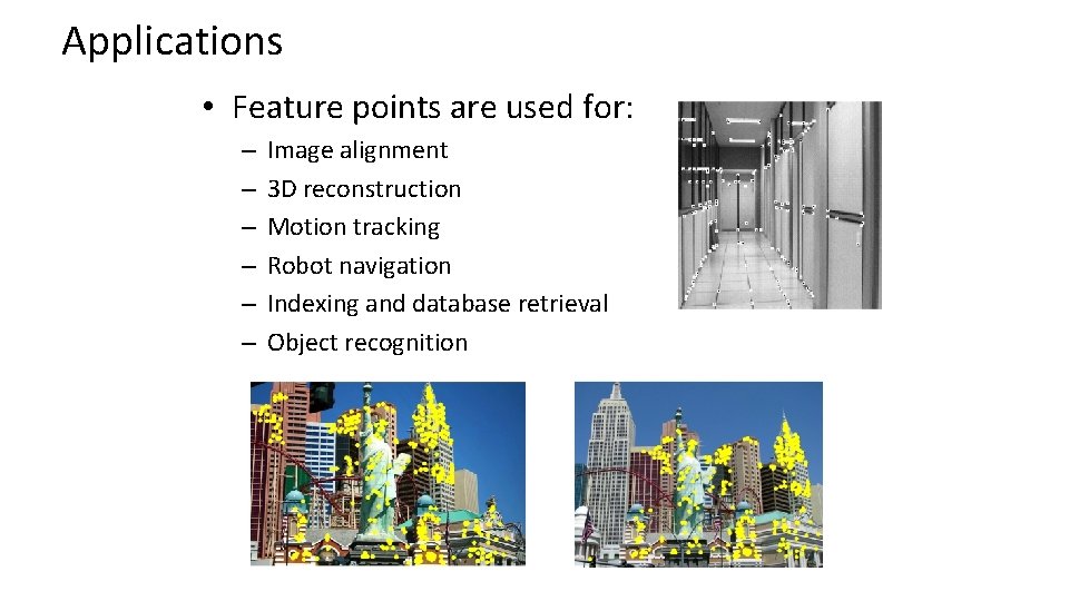
Applications • Feature points are used for: – – – Image alignment 3 D reconstruction Motion tracking Robot navigation Indexing and database retrieval Object recognition

Project 2: interest points and local features • Note: “interest points” = “keypoints”, also sometimes called “features”

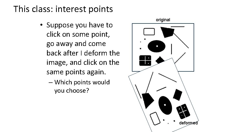
This class: interest points • Suppose you have to click on some point, go away and come back after I deform the image, and click on the same points again. original – Which points would you choose? deformed

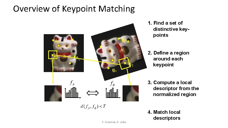
Overview of Keypoint Matching 1. Find a set of distinctive keypoints B 3 A 1 A 2 A 3 B 2 2. Define a region around each keypoint B 1 3. Compute a local descriptor from the normalized region K. Grauman, B. Leibe 4. Match local descriptors

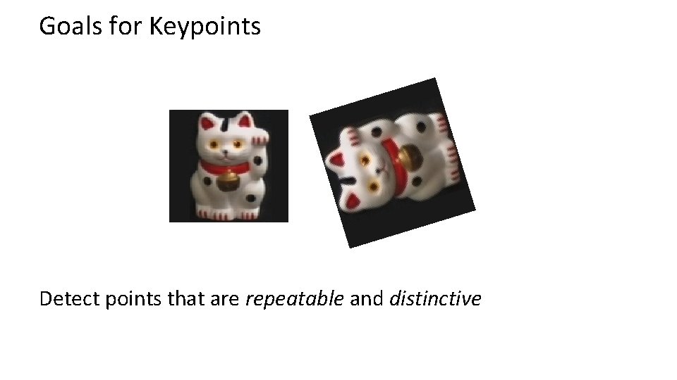
Goals for Keypoints Detect points that are repeatable and distinctive

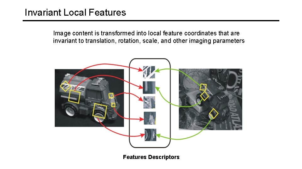
Invariant Local Features Image content is transformed into local feature coordinates that are invariant to translation, rotation, scale, and other imaging parameters Features Descriptors

Why extract features? • Motivation: panorama stitching • We have two images – how do we combine them?

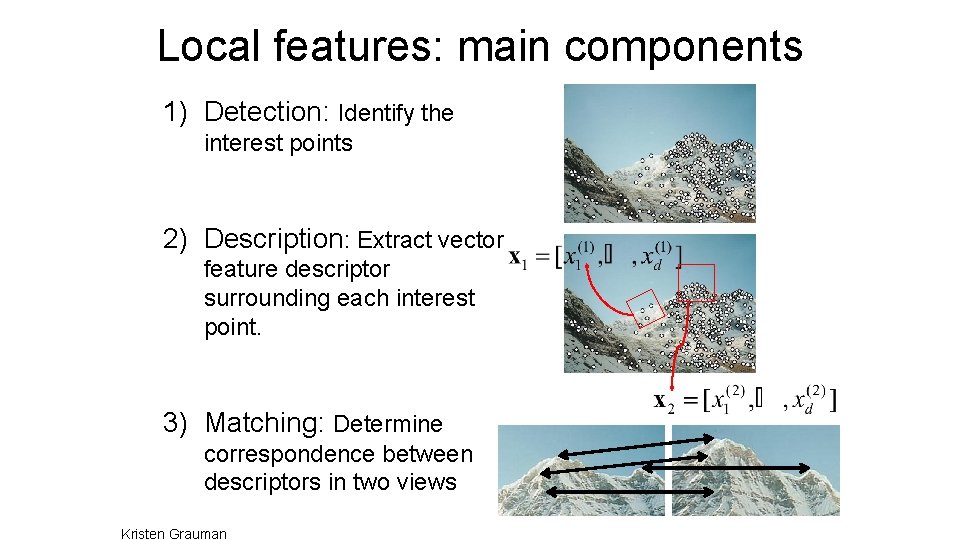
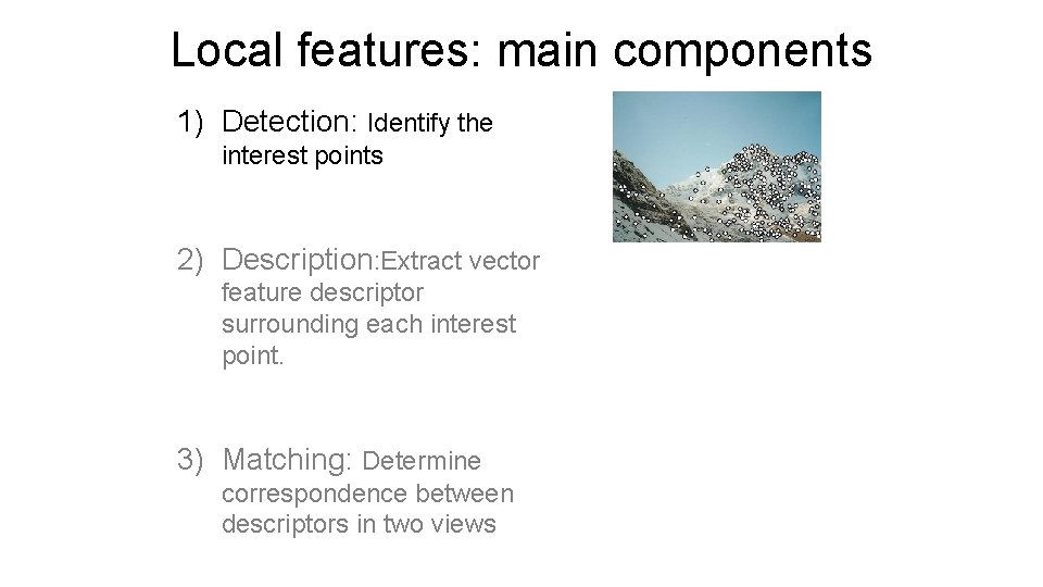
Local features: main components 1) Detection: Identify the interest points 2) Description: Extract vector feature descriptor surrounding each interest point. 3) Matching: Determine correspondence between descriptors in two views Kristen Grauman

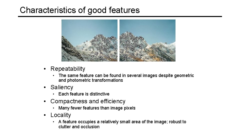
Characteristics of good features • Repeatability • The same feature can be found in several images despite geometric and photometric transformations • Saliency • Each feature is distinctive • Compactness and efficiency • Many fewer features than image pixels • Locality • A feature occupies a relatively small area of the image; robust to clutter and occlusion

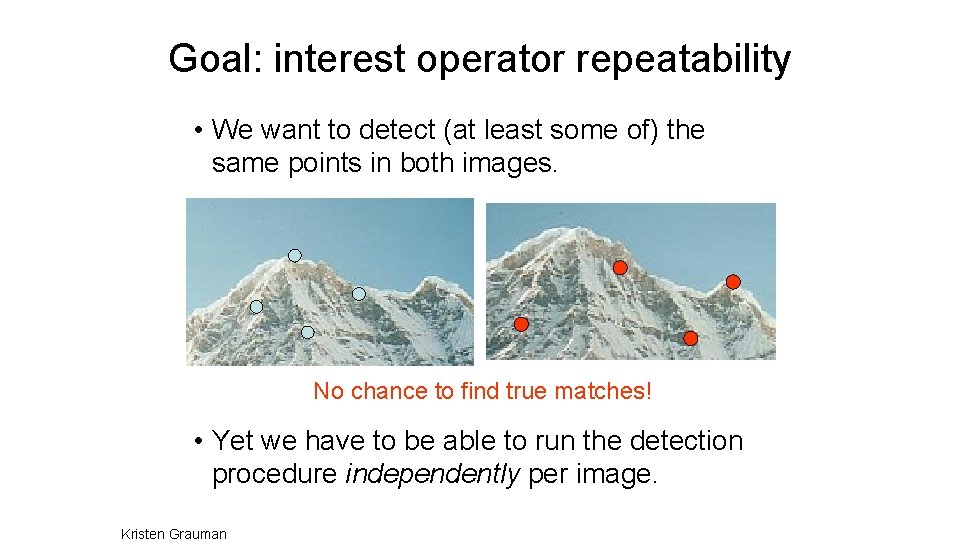
Goal: interest operator repeatability • We want to detect (at least some of) the same points in both images. No chance to find true matches! • Yet we have to be able to run the detection procedure independently per image. Kristen Grauman

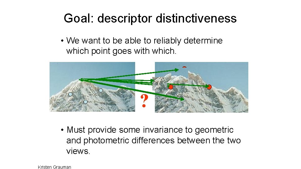
Goal: descriptor distinctiveness • We want to be able to reliably determine which point goes with which. ? • Must provide some invariance to geometric and photometric differences between the two views. Kristen Grauman

Local features: main components 1) Detection: Identify the interest points 2) Description: Extract vector feature descriptor surrounding each interest point. 3) Matching: Determine correspondence between descriptors in two views

Many Existing Detectors Available Hessian & Harris [Beaudet ‘ 78], [Harris ‘ 88] Laplacian, Do. G [Lindeberg ‘ 98], [Lowe 1999] Harris-/Hessian-Laplace [Mikolajczyk & Schmid ‘ 01] Harris-/Hessian-Affine[Mikolajczyk & Schmid ‘ 04] EBR and IBR [Tuytelaars & Van Gool ‘ 04] MSER [Matas ‘ 02] Salient Regions [Kadir & Brady ‘ 01] Others… K. Grauman, B. Leibe

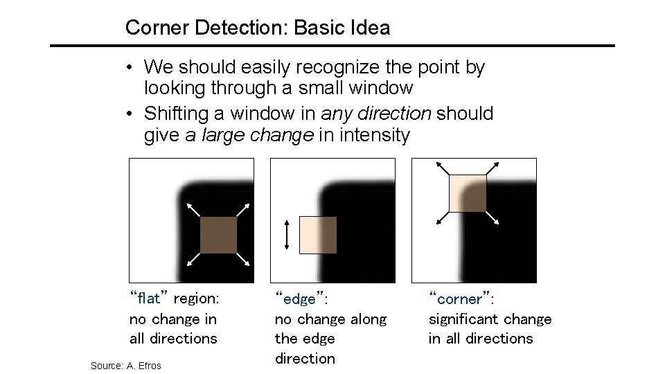
Corner Detection: Basic Idea • We should easily recognize the point by looking through a small window • Shifting a window in any direction should give a large change in intensity “flat” region: no change in all directions Source: A. Efros “edge”: no change along the edge direction “corner”: significant change in all directions

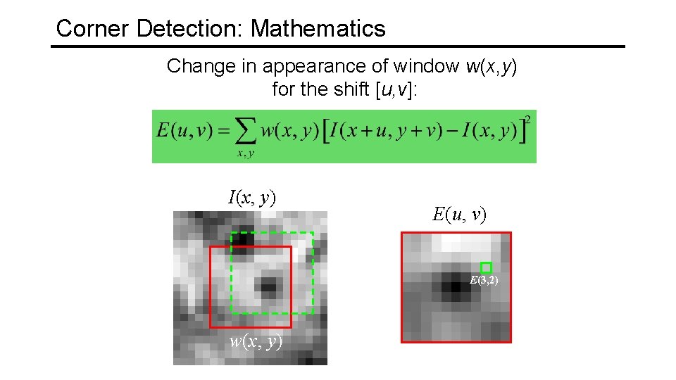
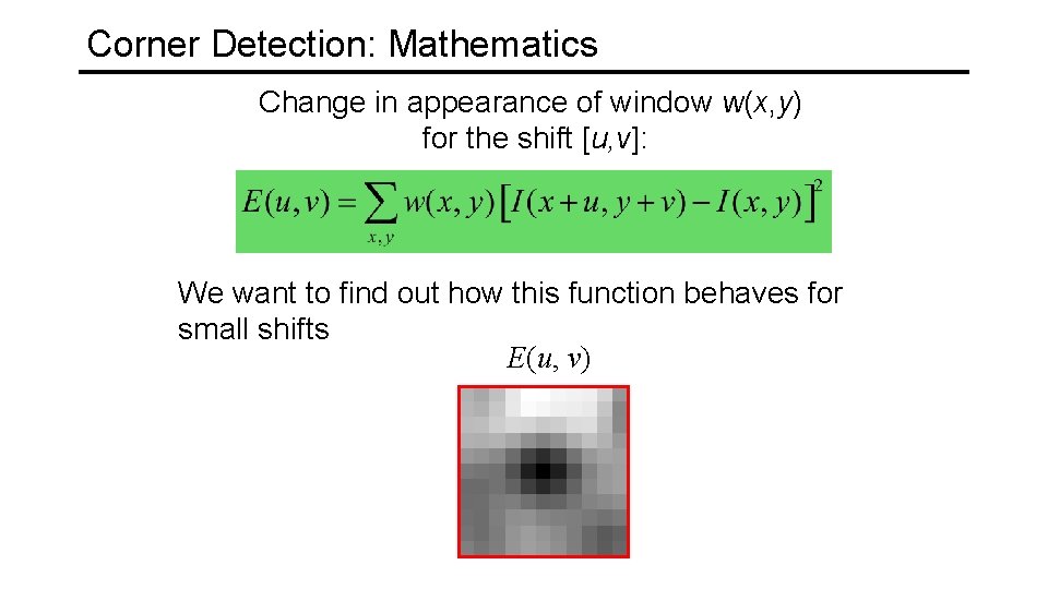
Corner Detection: Mathematics Change in appearance of window w(x, y) for the shift [u, v]: I(x, y) E(u, v) E(3, 2) w(x, y)

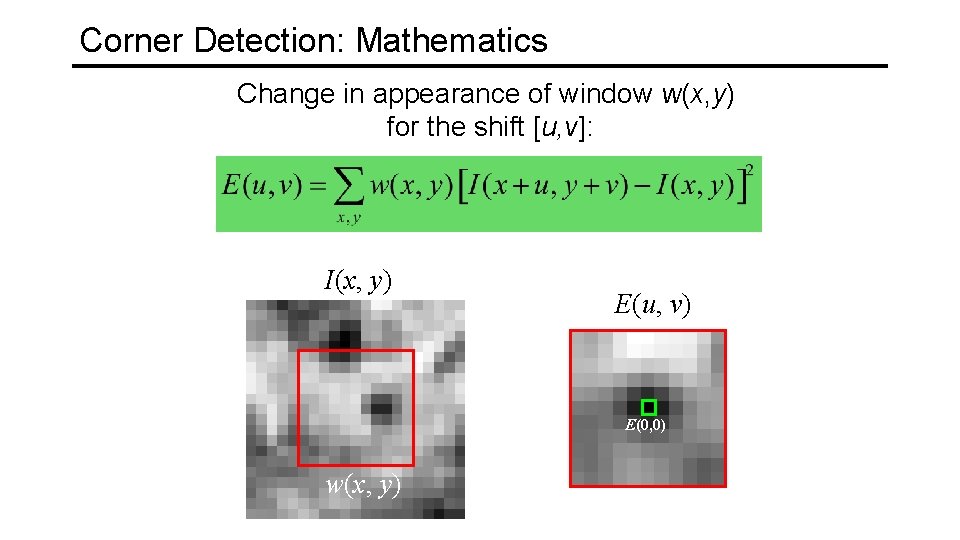
Corner Detection: Mathematics Change in appearance of window w(x, y) for the shift [u, v]: I(x, y) E(u, v) E(0, 0) w(x, y)

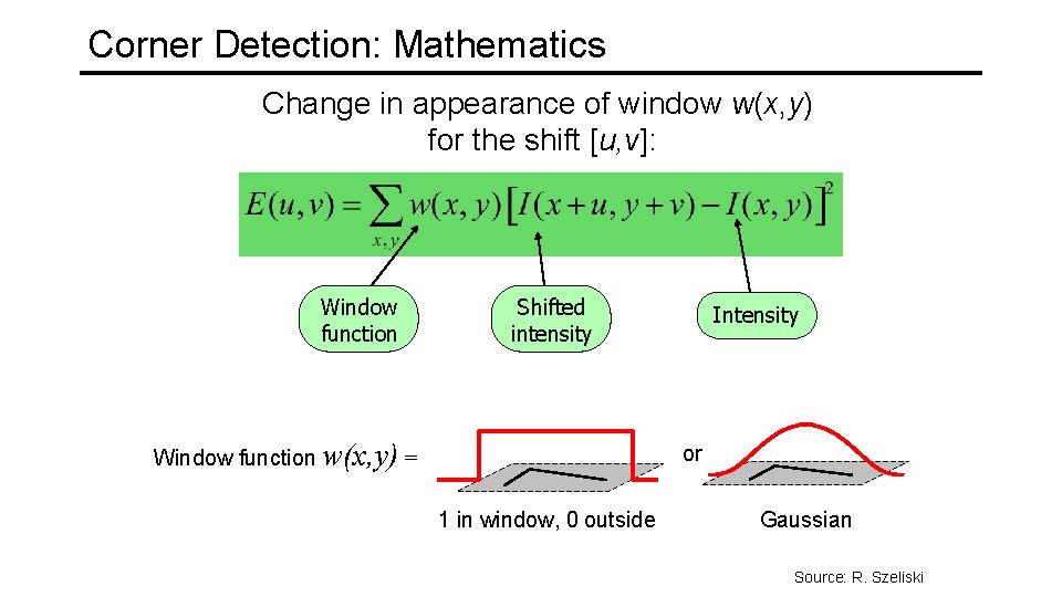
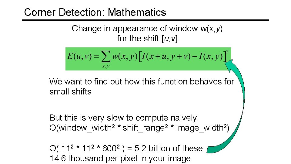
Corner Detection: Mathematics Change in appearance of window w(x, y) for the shift [u, v]: Window function Shifted intensity Window function w(x, y) = Intensity or 1 in window, 0 outside Gaussian Source: R. Szeliski

Corner Detection: Mathematics Change in appearance of window w(x, y) for the shift [u, v]: We want to find out how this function behaves for small shifts E(u, v)

Corner Detection: Mathematics Change in appearance of window w(x, y) for the shift [u, v]: We want to find out how this function behaves for small shifts But this is very slow to compute naively. O(window_width 2 * shift_range 2 * image_width 2) O( 112 * 6002 ) = 5. 2 billion of these 14. 6 thousand per pixel in your image

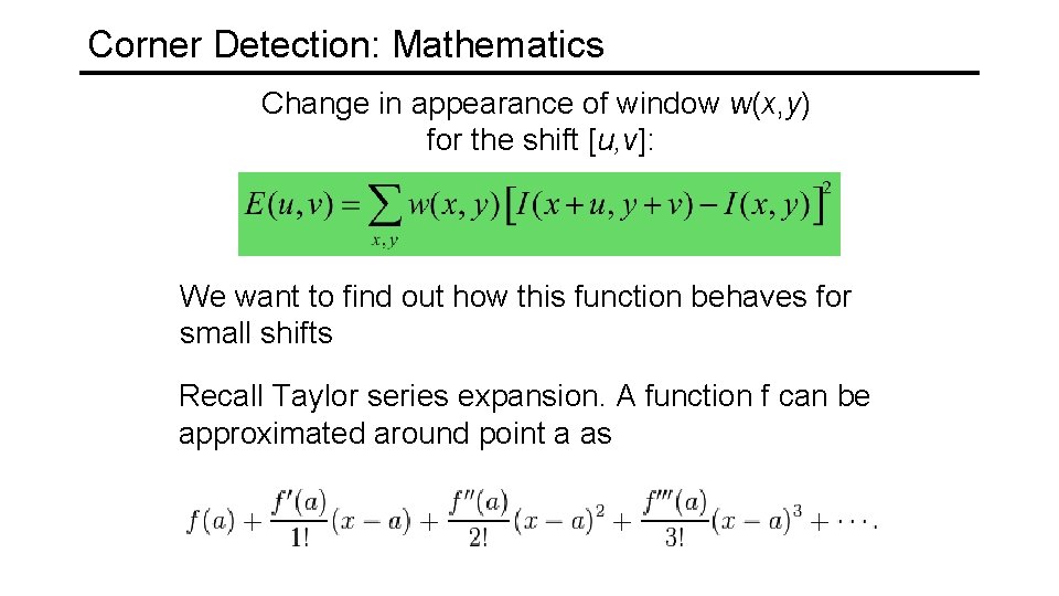
Corner Detection: Mathematics Change in appearance of window w(x, y) for the shift [u, v]: We want to find out how this function behaves for small shifts Recall Taylor series expansion. A function f can be approximated around point a as

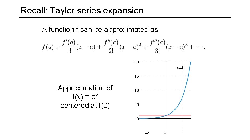
Recall: Taylor series expansion A function f can be approximated as Approximation of f(x) = ex centered at f(0)

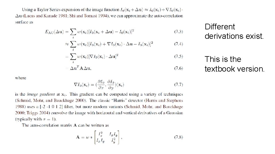
Different derivations exist. This is the textbook version.

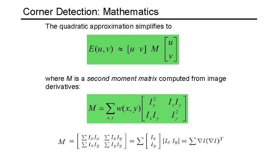
Corner Detection: Mathematics The quadratic approximation simplifies to where M is a second moment matrix computed from image derivatives: M

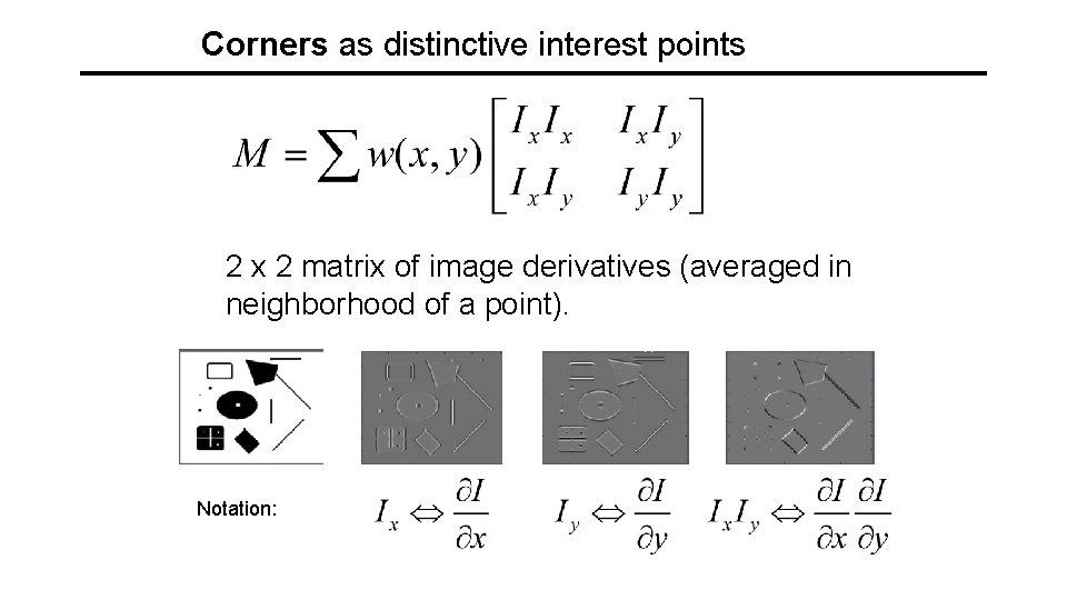
Corners as distinctive interest points 2 x 2 matrix of image derivatives (averaged in neighborhood of a point). Notation:

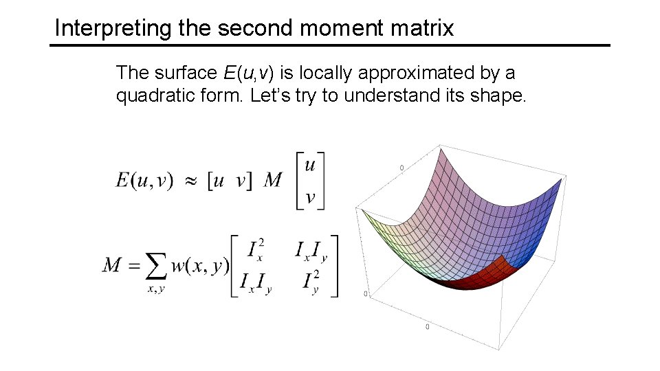
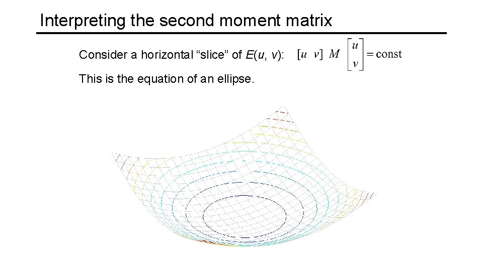
Interpreting the second moment matrix The surface E(u, v) is locally approximated by a quadratic form. Let’s try to understand its shape.

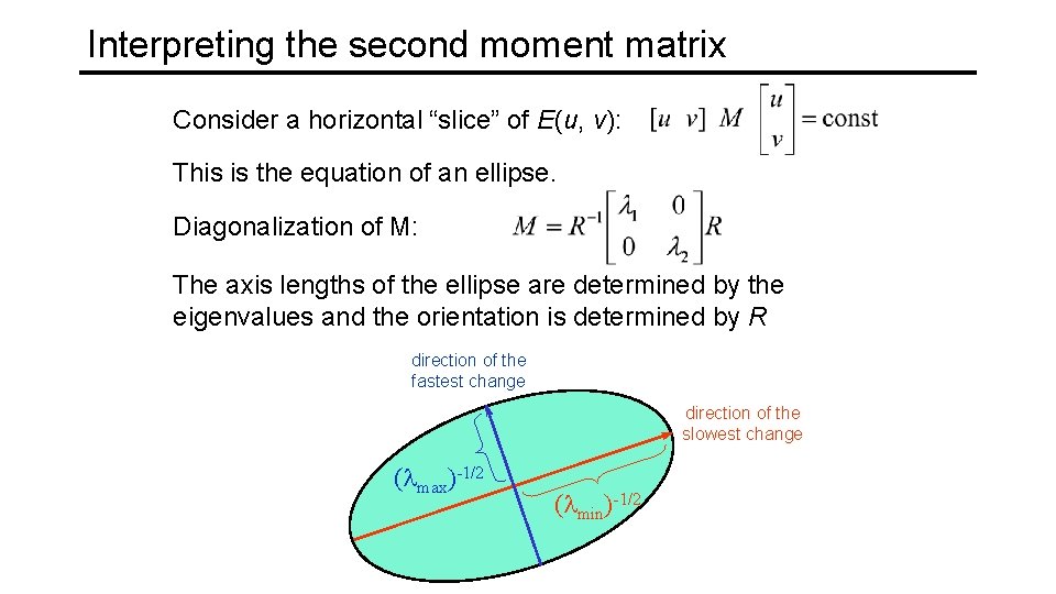
Interpreting the second moment matrix Consider a horizontal “slice” of E(u, v): This is the equation of an ellipse.

Interpreting the second moment matrix Consider a horizontal “slice” of E(u, v): This is the equation of an ellipse. Diagonalization of M: The axis lengths of the ellipse are determined by the eigenvalues and the orientation is determined by R direction of the fastest change direction of the slowest change ( max)-1/2 ( min)-1/2

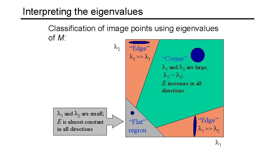
Interpreting the eigenvalues Classification of image points using eigenvalues of M: 2 “Edge” 2 >> 1 “Corner” 1 and 2 are large, 1 ~ 2; E increases in all directions 1 and 2 are small; E is almost constant in all directions “Flat” region “Edge” 1 >> 2 1

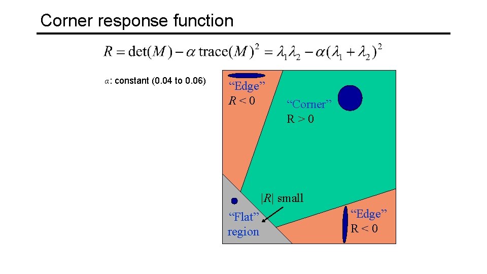
Corner response function α: constant (0. 04 to 0. 06) “Edge” R<0 “Corner” R>0 |R| small “Flat” region “Edge” R<0

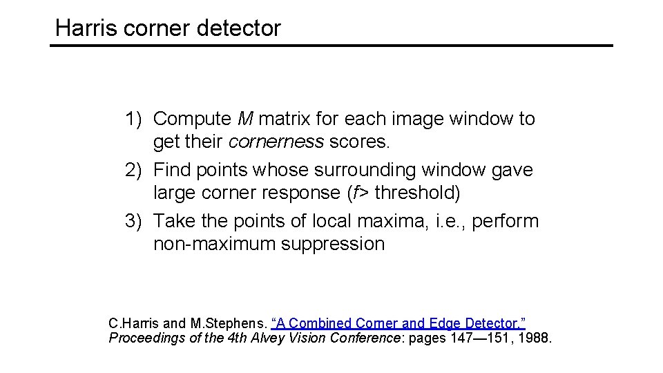
Harris corner detector 1) Compute M matrix for each image window to get their cornerness scores. 2) Find points whose surrounding window gave large corner response (f> threshold) 3) Take the points of local maxima, i. e. , perform non-maximum suppression C. Harris and M. Stephens. “A Combined Corner and Edge Detector. ” Proceedings of the 4 th Alvey Vision Conference: pages 147— 151, 1988.

Harris Detector [Harris 88] • Second moment matrix 1. Image derivatives (optionally, blur first) Ix Iy Ix 2 Iy 2 Ix Iy g(Ix 2) g(Iy 2) g(Ix. Iy) 2. Square of derivatives 3. Gaussian filter g(s. I) 4. Cornerness function – both eigenvalues are strong 5. Non-maxima suppression har 65

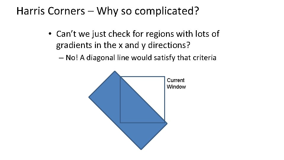
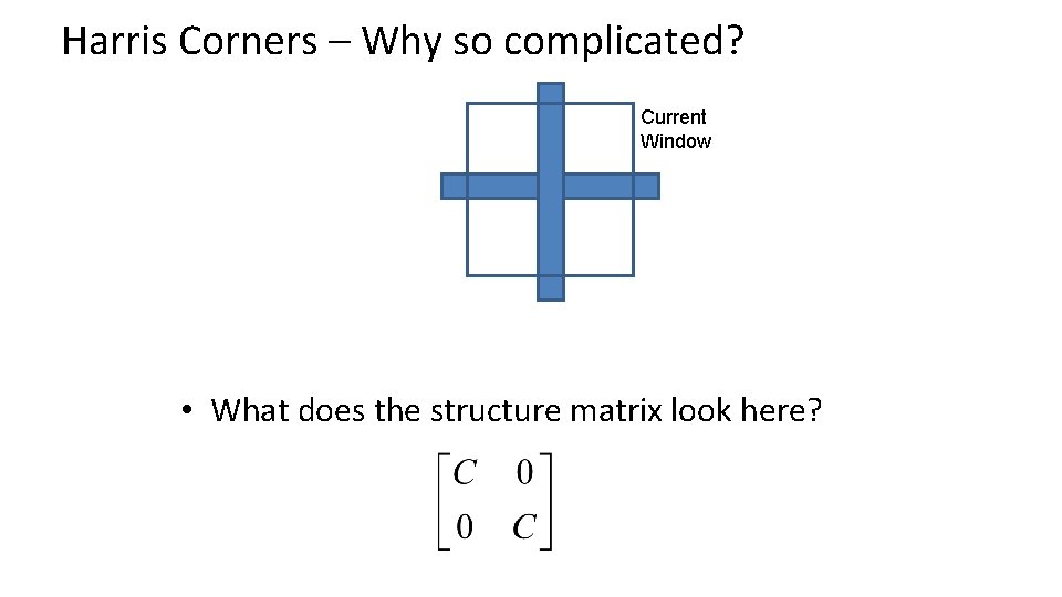
Harris Corners – Why so complicated? • Can’t we just check for regions with lots of gradients in the x and y directions? – No! A diagonal line would satisfy that criteria Current Window

Harris Detector [Harris 88] • Second moment matrix 1. Image derivatives (optionally, blur first) Ix Iy Ix 2 Iy 2 Ix Iy g(Ix 2) g(Iy 2) g(Ix. Iy) 2. Square of derivatives 3. Gaussian filter g(s. I) 4. Cornerness function – both eigenvalues are strong 5. Non-maxima suppression har 67

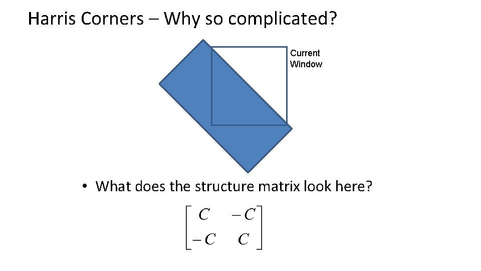
Harris Corners – Why so complicated? Current Window • What does the structure matrix look here?

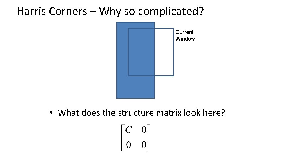
Harris Corners – Why so complicated? Current Window • What does the structure matrix look here?

Harris Corners – Why so complicated? Current Window • What does the structure matrix look here?

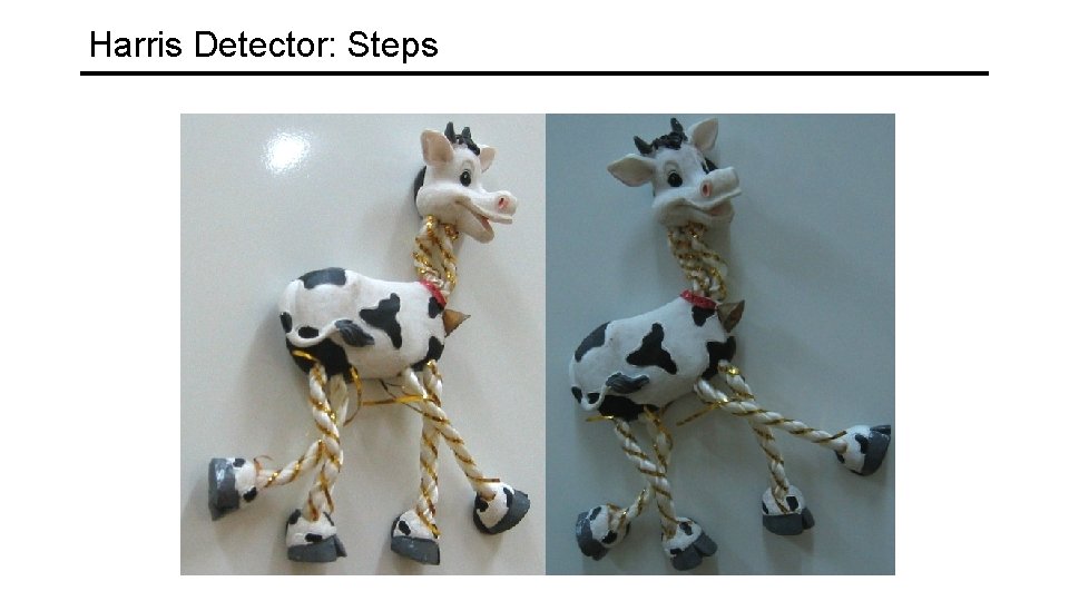
Harris Detector: Steps

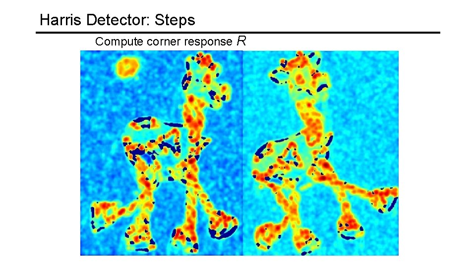
Harris Detector: Steps Compute corner response R

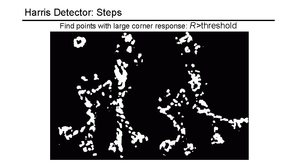
Harris Detector: Steps Find points with large corner response: R>threshold

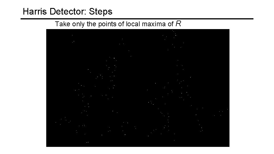
Harris Detector: Steps Take only the points of local maxima of R

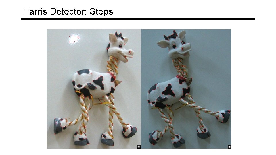
Harris Detector: Steps

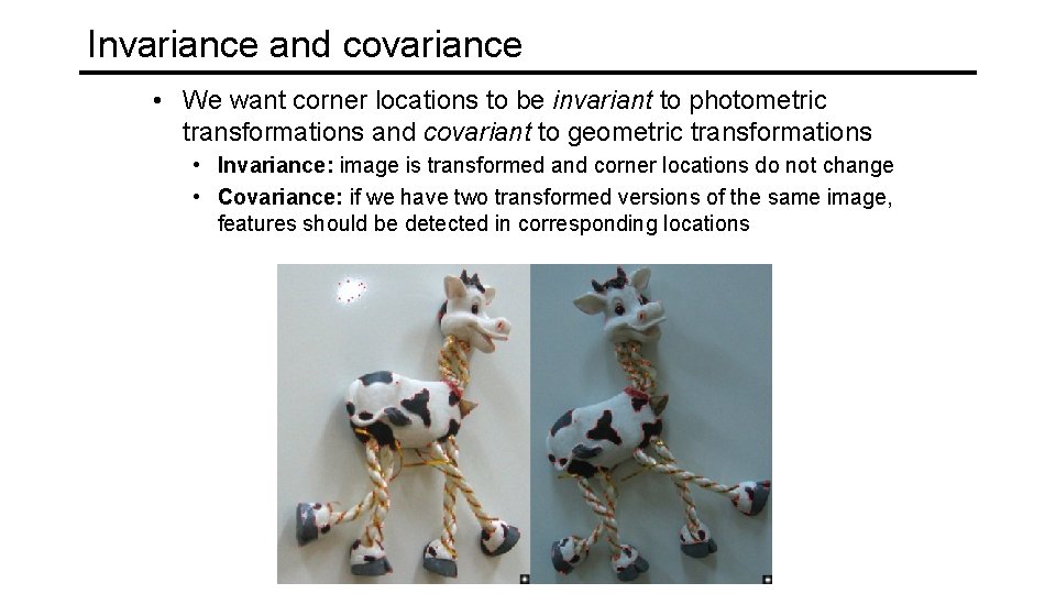
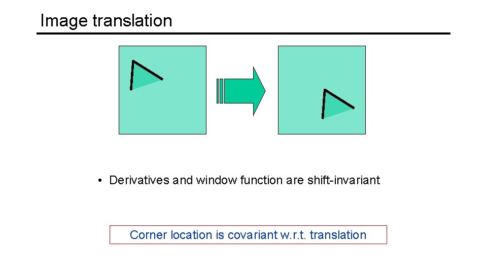
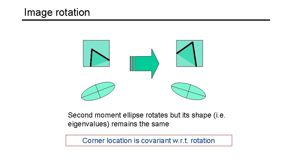
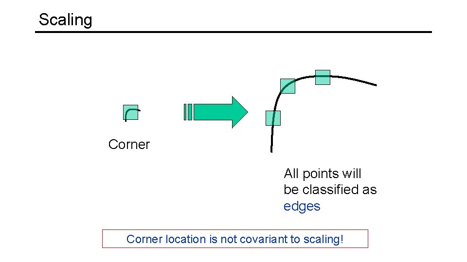
Invariance and covariance • We want corner locations to be invariant to photometric transformations and covariant to geometric transformations • Invariance: image is transformed and corner locations do not change • Covariance: if we have two transformed versions of the same image, features should be detected in corresponding locations

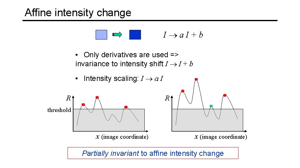
Affine intensity change I a. I+b • Only derivatives are used => invariance to intensity shift I I + b • Intensity scaling: I a I R R threshold x (image coordinate) Partially invariant to affine intensity change

Image translation • Derivatives and window function are shift-invariant Corner location is covariant w. r. t. translation

Image rotation Second moment ellipse rotates but its shape (i. e. eigenvalues) remains the same Corner location is covariant w. r. t. rotation

Scaling Corner All points will be classified as edges Corner location is not covariant to scaling!