Recap last Thursday Linear Regression What is it

• Recap last Thursday • Linear Regression – What is it? Why do we do it? – How to build it? – Running it in Python • LASSO – What is it? Why do we do it? – How to build it? – Running it in Python

Logistic Regression

Why Logistic Regression? § There are many important research topics for which the dependent variable is "limited. " § For example: voting, conversion, and participation data is not continuous or distributed normally. § Binary logistic regression is a type of regression analysis where the dependent variable is a dummy variable: coded 0 (did not happen) or 1(did happen)

Car Prices (Revisited)

Car Prices (Cont)

Car Prices Model • Fit a linear model to the data – B 0 = 19, 528 – B 1 = -0. 195 • How much is a car with 100, 000 miles worth? – $28 • How much is a car with 200, 000 miles worth? – -$19, 472

Transforming • Y = B 0 + B 1 x by B 1 - if you change x by 1, expect Y to change • log(Y) = B 0 + B 1 x - if you change x by 1, expect Y to change by 100 * B 1 percent • Y = B 0 + B 1 log(x) - if you change x by 1%, expect Y to change by B 1/100 units • log(Y) = B 0 + B 1 log(x) - if you change x by 1%, expect Y to change by B 1 %

Car Prices Model - Logged • Logging our prices, we can refit our model (i. e. log(Y) = B 0 + B 1 * X) Y = e B 0 + B 1 * X – B 0 = 9. 839 – B 1 = -0. 00001929 • How much is a car with 100, 000 miles worth? – $2805 • How much is a car with 200, 000 miles worth? – $419

Transforming Data • Transforming data can help model more accurately and using tools such as OLS or MLE (maximum likelihood estimators) • Suppose we have voting data. 1 for voted and 0 for non-voting. We also have age. How could we model the likelihood to vote given someone’s age?

Voting by Age

Voting Example (cont. )

Voting Example (cont. )

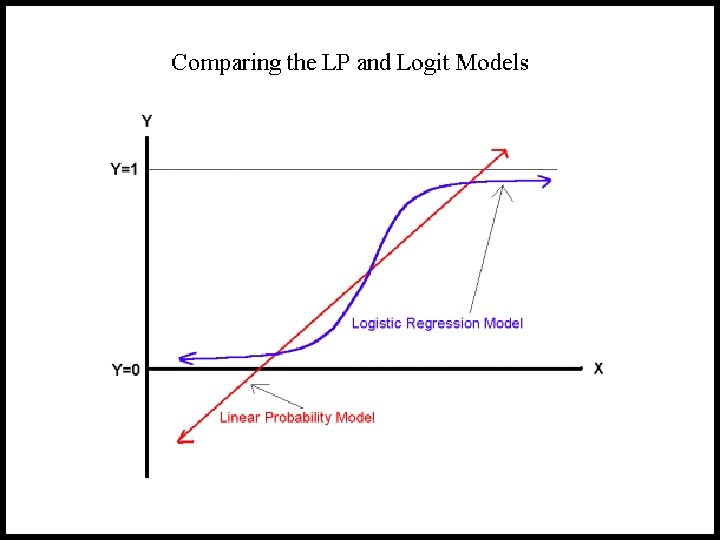
The Logistic Regression Model The "logit" model solves these problems: ln[p/(1 -p)] = + X + e § p is the probability that the event Y occurs, p(Y=1) § p/(1 -p) is the "odds ratio" § ln[p/(1 -p)] is the log odds ratio, or "logit"

More: § The logistic distribution constrains the estimated probabilities to lie between 0 and 1. § The estimated probability is: p = 1/[1 + exp(- - X)] § if you let + X =0, then p =. 50 § as + X gets really big, p approaches 1 § as + X gets really negative, p approaches 0

Interpreting Coefficients § Since: ln[p/(1 -p)] = + X + e The slope coefficient ( ) is interpreted as the rate of change in the "log odds" as X changes … not very useful.

• An interpretation of the logit coefficient which is usually more intuitive is the "odds ratio" • Since: [p/(1 -p)] = exp( + X) exp( ) is the effect of the independent variable on the "odds ratio” • exp( ) = probability of the “average person” • exp( ) = times more likely

Demo

LASSO (Least Absolute Shrinkage and Selection Operator)

Improving OLS • We may want to improve the simple linear model by replacing OLS estimation with some alternative fitting procedure. • Recall OLS estimators are the have the least variance for unbiased estimators. • In that case, why use an alternative fitting procedure? – Prediction Accuracy – Model Interpretability

Bias/Variance Trade-Off • There is always a trade-off between variance and bias (i. e. the more variance we introduce, the less bias. Similarly, the more bias, the less variance)

Bias/Variance (Cont. ) • As models become more complex (more terms included), local structure/curvature can be picked up. • However, coefficient estimates are highly volatile and have more variance as more terms are included.

Bias/Variance (Cont. ) • Carefully selected features can improve model accuracy, but adding too many can lead to overfitting. – Overfitted models describe random error or noise instead of any underlying relationship. – They generally have poor predictive performance on test data. • Overfitted models will usually describe the training data set very well. • However, a brand new dataset collected from the same population may not fit this particular curve well at all.

Example: 10 -Degree polynomials

Example: 10 -Degree polynomials

Example: 10 -Degree polynomials

Example: 10 -Degree polynomials

Example: 10 -Degree polynomials

Prediction Accuracy • If we add bias, we can minimize or reduce some of the variance • How can we add bias? – One way to do this is to remove some of our terms. • What are some methods for removing some of the terms? – P-values – AIC/BIC

Problems with p-values • With p-values, we check to see if a Bn is non-0. If it is 0, we remove it from the model and create a new model. • With large n, many p-values will be significant even if there is little to no effect. • Increased power of large samples means you can detect smaller, subtler and more complex effects but this can cause overfitting/overcomplexity.

Problems with AIC/BIC • AIC/BIC are measures of model fit with a penalty for the number of parameters. • Would need to explore all models “by hand” • Too many models to do this even computationally • 2^p models to evaluate

Model Interpretability • When we have a large number of predictors in the model, there will generally be many that have little or no effect on the response. • Including such irrelevant variable leads to unnecessary complexity. • Leaving these variables in the model makes it harder to see the effect of the important variables. • The model would be easier to interpret by removing (i. e. setting the coefficients to zero) the unimportant variables.

Shrinkage (Regularization) Methods • The subset selection methods use OLS to fit a linear model that contains a subset of the predictors. • As an alternative, we can fit a model containing all p predictors using a technique that constrains or regularizes the coefficient estimates (i. e. shrinks the coefficient estimates towards zero). • Regularization is our first weapon to combat overfitting. • It may not be immediately obvious why such a constraint should improve the fit, but it turns out that shrinking the coefficient estimates can significantly reduce their variance.

The Lasso • The lasso coefficients minimize the quantity: • The key difference from OLS and lasso is the lasso uses a penalty for including larger coefficients. This has the effect of forcing some of the coefficients to be exactly equal to zero when the tuning parameter λ is sufficiently large. • Thus, the lasso performs variable/feature selection.

The Lasso (cont. ) • The standard OLS coefficient estimates are scale equivariant. • However, the lasso regression coefficient estimates can change substantially when multiplying a given predictor by a constant, due to the sum-of-absolute-values-of-thecoefficients term in the penalty part of the lasso regression objective function. • Thus, it is best to apply lasso regression after standardizing the predictors:

The Lasso (cont. ) • Notice that the solution is indexed by the paramter λ. – So for each λ, we have a solution – The λ’s trace out a path of solutions (see next slide) • λ is the shrinkage parameter – λ controls the size of the coefficients – λ controls the amount of regularization – As λ 0, we obtain the OLS solution – As λ 1, we obtain βlasso=0 (intercept only model)

The Lasso (cont. ) § § When λ = 0, then the lasso simply gives the OLS fit. When λ becomes sufficiently large, the lasso gives the null model in which all coefficient estimates equal zero.

Other Shrinkage Methods • Ridge regression = • Elastic Net = combination of ridge and lasso penalty (with 2 different lambdas) • One significant problem of ridge regression is that the penalty term will never force any of the coefficients to be exactly zero. • Thus, the final model will include all p predictors, which creates a challenge in model interpretation

Lasso vs. Ridge Regression • The lasso has a major advantage over ridge regression, in that it produces simpler and more interpretable models that involved only a subset of predictors. • The lasso leads to qualitatively similar behavior to ridge regression, in that as λ increases, the variance decreases and the bias increases. • The lasso can generate more accurate predictions compared to ridge regression. • Cross-validation can be used in order to determine which approach is better on a particular data set.

Selecting the Tuning Parameter λ • As for subset selection, for ridge regression and lasso we require a method to determine which of the models under consideration in best; thus, we required a method selecting a value for the tuning parameter λ or equivalently, the value of the constraint s. • Select a grid of potential values; use cross-validation to estimate the error rate on test data (for each value of λ) and select the value that gives the smallest error rate. • Finally, the model is re-fit using all of the variable observations and the selected value of the tuning parameter λ.

Cross-Validation (k-fold) • Original sample is partitioned into K subsamples • 1 subsample is used for validation, K-1 is used for training • Process (e. g. best fit, minimized loss function, etc. ) conducted, then repeated K times • Results are then averaged to produce final result • 10 fold is most commonly used (also 20)

Demo