Recap 1 2 1 in EB Property insurance

Recap (1. 2. 1 in EB) • Property insurance is economic responsibility for incidents such as fires and accidents passed on to an insurer against a fee • The contract, known as a policy, releases claims when such events occur • A central quantity is the total claim X amassed during a certain period of time (typically a year)

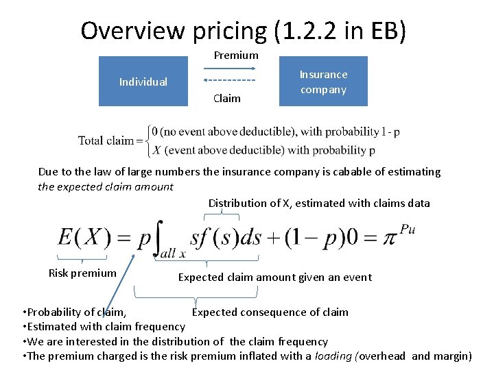
Overview pricing (1. 2. 2 in EB) Premium Individual Claim Insurance company Due to the law of large numbers the insurance company is cabable of estimating the expected claim amount Distribution of X, estimated with claims data Risk premium Expected claim amount given an event • Probability of claim, Expected consequence of claim • Estimated with claim frequency • We are interested in the distribution of the claim frequency • The premium charged is the risk premium inflated with a loading (overhead and margin)

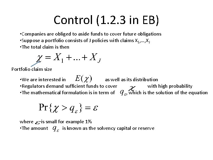
Control (1. 2. 3 in EB) • Companies are obliged to aside funds to cover future obligations • Suppose a portfolio consists of J policies with claims X 1, …, XJ • The total claim is then Portfolio claim size • We are interested in as well as its distribution • Regulators demand sufficient funds to cover with high probability • The mathematical formulation is in term of , which is the solution of the equation where is small for example 1% • The amount is known as the solvency capital or reserve

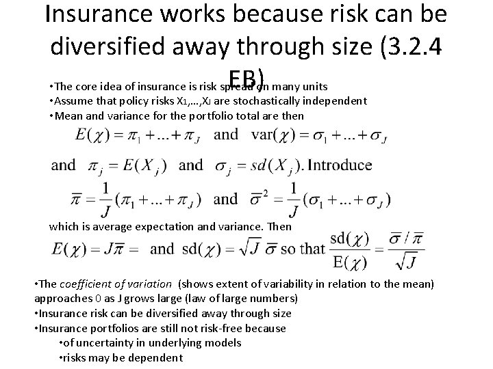
Insurance works because risk can be diversified away through size (3. 2. 4 EB)on many units • The core idea of insurance is risk spread • Assume that policy risks X 1, …, XJ are stochastically independent • Mean and variance for the portfolio total are then which is average expectation and variance. Then • The coefficient of variation (shows extent of variability in relation to the mean) approaches 0 as J grows large (law of large numbers) • Insurance risk can be diversified away through size • Insurance portfolios are still not risk-free because • of uncertainty in underlying models • risks may be dependent

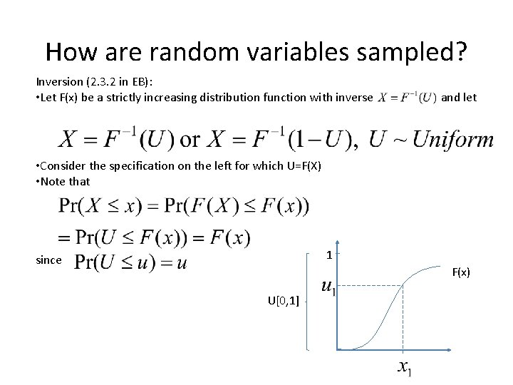
How are random variables sampled? Inversion (2. 3. 2 in EB): • Let F(x) be a strictly increasing distribution function with inverse and let • Consider the specification on the left for which U=F(X) • Note that 1 since F(x) U[0, 1]

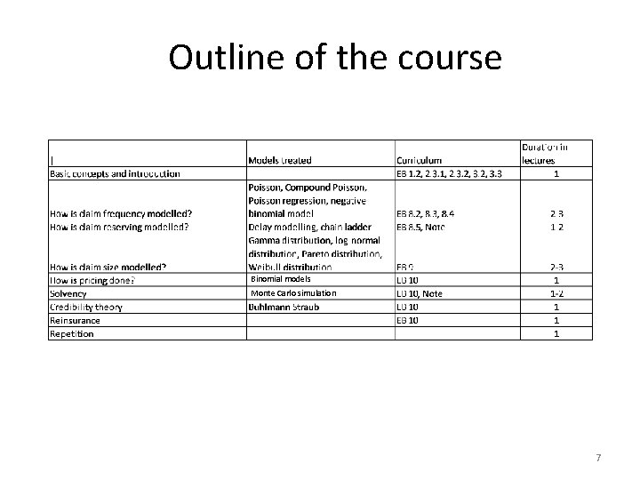
Outline of the course Binomial models Monte Carlo simulation 7

Course literature Curriculum: Chapter 1. 2, 2. 3. 1, 2. 3. 2, 2. 5, 3. 2, 3. 3 in EB Chapter 8, 9, 10 in EB Note on Chain Ladder Lecture notes by NFH Exercises The following book will be used (EB): Computation and Modelling in Insurance and Finance, Erik Bølviken, Cambridge University Press (2013) • Additions to the list above may occur during the course • Final curriculum will be posted on the course web site in due time Assignment must be approved to be able to participate in exame 8

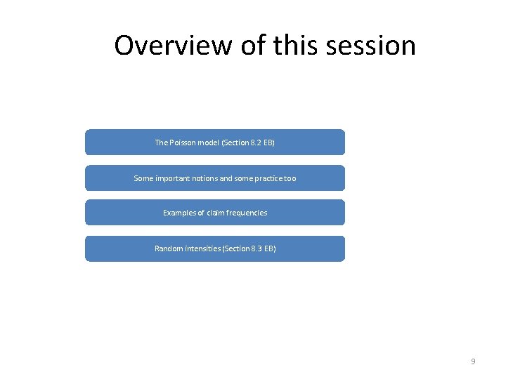
Overview of this session The Poisson model (Section 8. 2 EB) Some important notions and some practice too Examples of claim frequencies Random intensities (Section 8. 3 EB) 9

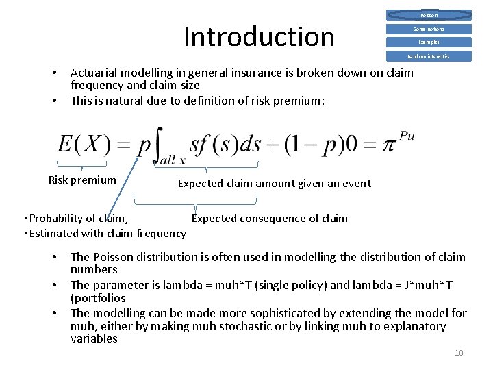
Introduction • • Poisson Some notions Examples Random intensities Actuarial modelling in general insurance is broken down on claim frequency and claim size This is natural due to definition of risk premium: Risk premium Expected claim amount given an event • Probability of claim, Expected consequence of claim • Estimated with claim frequency • • • The Poisson distribution is often used in modelling the distribution of claim numbers The parameter is lambda = muh*T (single policy) and lambda = J*muh*T (portfolios The modelling can be made more sophisticated by extending the model for muh, either by making muh stochastic or by linking muh to explanatory variables 10

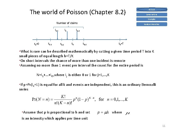
The world of Poisson (Chapter 8. 2) Poisson Some notions Examples Number of claims Ik Ik-1 t 0=0 tk-2 tk-1 Random intensities Ik+1 tk tk+1 tk=T • What is rare can be described mathematically by cutting a given time period T into K small pieces of equal length h=T/K • On short intervals the chance of more than one incident is remote • Assuming no more than 1 event per interval the count for the entire period is N=I 1+. . . +IK , where Ij is either 0 or 1 for j=1, . . . , K • If p=Pr(Ik=1) is equal for all k and events are independent, this is an ordinary Bernoulli series • Assume that p is proportional to h and set is an intensity which applies per time unit where 11

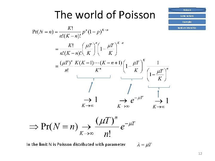
The world of Poisson Some notions Examples Random intensities In the limit N is Poisson distributed with parameter 12

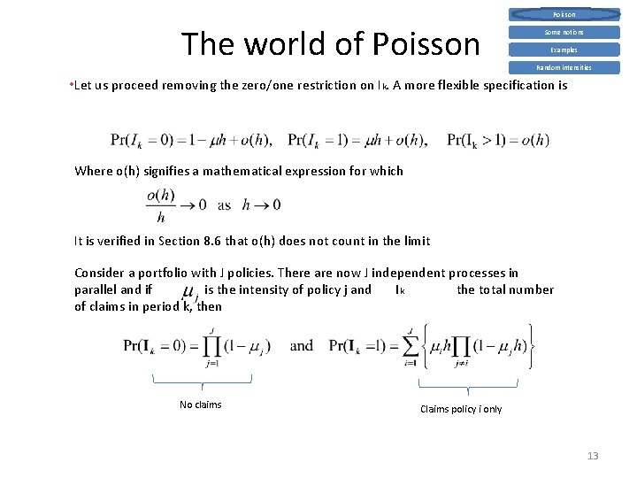
Poisson The world of Poisson Some notions Examples Random intensities • Let us proceed removing the zero/one restriction on Ik. A more flexible specification is Where o(h) signifies a mathematical expression for which It is verified in Section 8. 6 that o(h) does not count in the limit Consider a portfolio with J policies. There are now J independent processes in parallel and if is the intensity of policy j and Ik the total number of claims in period k, then No claims Claims policy i only 13

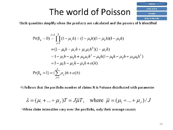
Poisson The world of Poisson Some notions Examples Random intensities • Both quanities simplify when the products are calculated and the powers of h identified • It follows that the portfolio number of claims N is Poisson distributed with parameter • When claim intensities vary over the portfolio, only their average counts 14

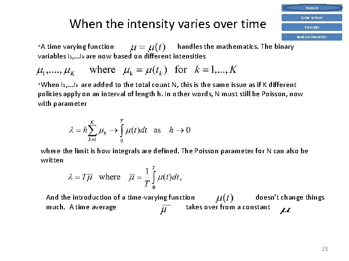
Poisson When the intensity varies over time Some notions Examples Random intensities • A time varying function handles the mathematics. The binary variables I 1, . . . Ik are now based on different intensities • When I 1, . . . Ik are added to the total count N, this is the same issue as if K different policies apply on an interval of length h. In other words, N must still be Poisson, now with parameter where the limit is how integrals are defined. The Poisson parameter for N can also be written And the introduction of a time-varying function doesn’t change things much. A time average takes over from a constant 15

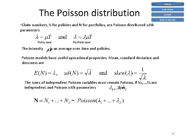
Poisson The Poisson distribution Some notions Examples Random intensities • Claim numbers, N for policies and N for portfolios, are Poisson distributed with parameters Policy level The intensity Portfolio level is an average over time and policies. Poisson models have useful operational properties. Mean, standard deviation and skewness are The sums of independent Poisson variables must remain Poisson, if N 1, . . . , NJ are independent and Poisson with parameters then ~ 16

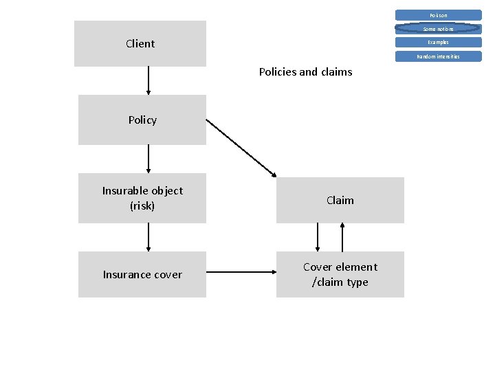
Poisson Some notions Client Examples Random intensities Policies and claims Policy Insurable object (risk) Claim Insurance cover Cover element /claim type

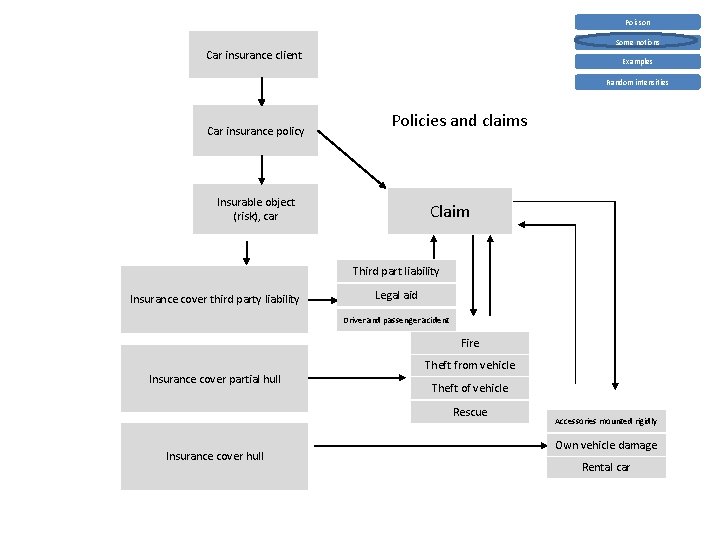
Poisson Some notions Car insurance client Examples Random intensities Car insurance policy Policies and claims Insurable object (risk), car Claim Third part liability Insurance cover third party liability Legal aid Driver and passenger acident Fire Insurance cover partial hull Theft from vehicle Theft of vehicle Rescue Insurance cover hull Accessories mounted rigidly Own vehicle damage Rental car

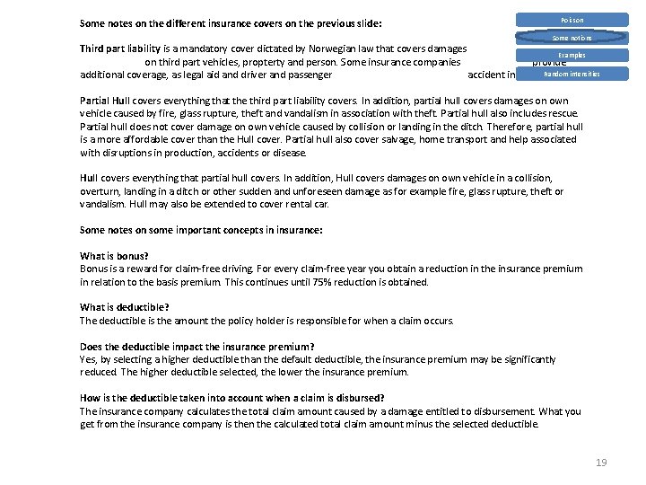
Poisson Some notes on the different insurance covers on the previous slide: Some notions Third part liability is a mandatory cover dictated by Norwegian law that covers damages Examples on third part vehicles, propterty and person. Some insurance companies provide Random intensities additional coverage, as legal aid and driver and passenger accident insurance. Partial Hull covers everything that the third part liability covers. In addition, partial hull covers damages on own vehicle caused by fire, glass rupture, theft and vandalism in association with theft. Partial hull also includes rescue. Partial hull does not cover damage on own vehicle caused by collision or landing in the ditch. Therefore, partial hull is a more affordable cover than the Hull cover. Partial hull also cover salvage, home transport and help associated with disruptions in production, accidents or disease. Hull covers everything that partial hull covers. In addition, Hull covers damages on own vehicle in a collision, overturn, landing in a ditch or other sudden and unforeseen damage as for example fire, glass rupture, theft or vandalism. Hull may also be extended to cover rental car. Some notes on some important concepts in insurance: What is bonus? Bonus is a reward for claim-free driving. For every claim-free year you obtain a reduction in the insurance premium in relation to the basis premium. This continues until 75% reduction is obtained. What is deductible? The deductible is the amount the policy holder is responsible for when a claim occurs. Does the deductible impact the insurance premium? Yes, by selecting a higher deductible than the default deductible, the insurance premium may be significantly reduced. The higher deductible selected, the lower the insurance premium. How is the deductible taken into account when a claim is disbursed? The insurance company calculates the total claim amount caused by a damage entitled to disbursement. What you get from the insurance company is then the calculated total claim amount minus the selected deductible. 19

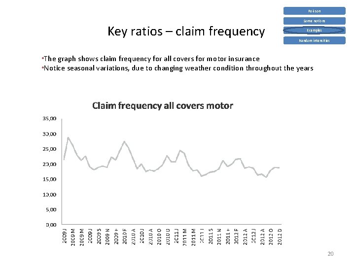
Poisson Key ratios – claim frequency Some notions Examples Random intensities • The graph shows claim frequency for all covers for motor insurance • Notice seasonal variations, due to changing weather condition throughout the years 20

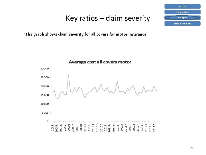
Poisson Key ratios – claim severity Some notions Examples Random intensities • The graph shows claim severity for all covers for motor insurance 21

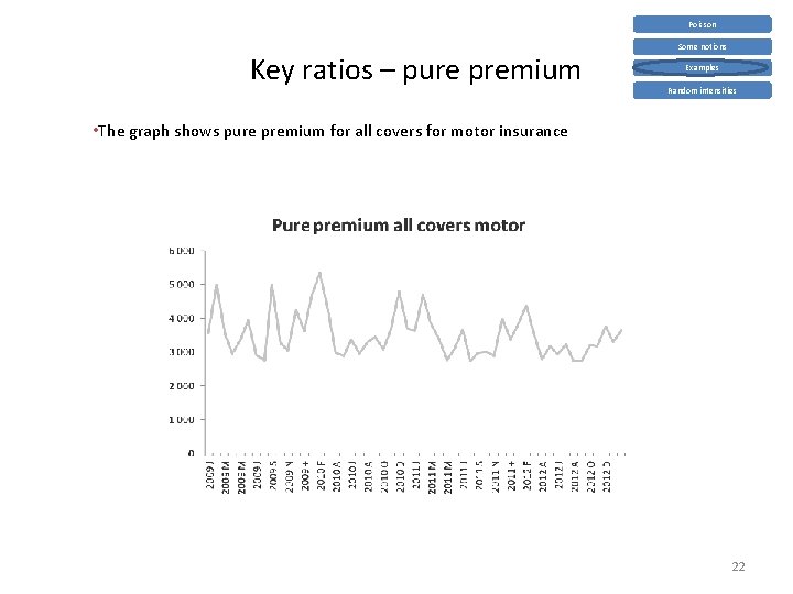
Poisson Key ratios – pure premium Some notions Examples Random intensities • The graph shows pure premium for all covers for motor insurance 22

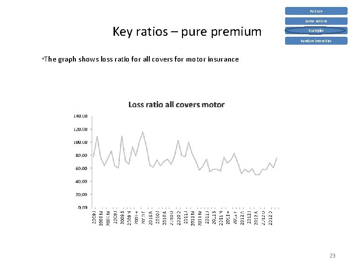
Poisson Key ratios – pure premium Some notions Examples Random intensities • The graph shows loss ratio for all covers for motor insurance 23

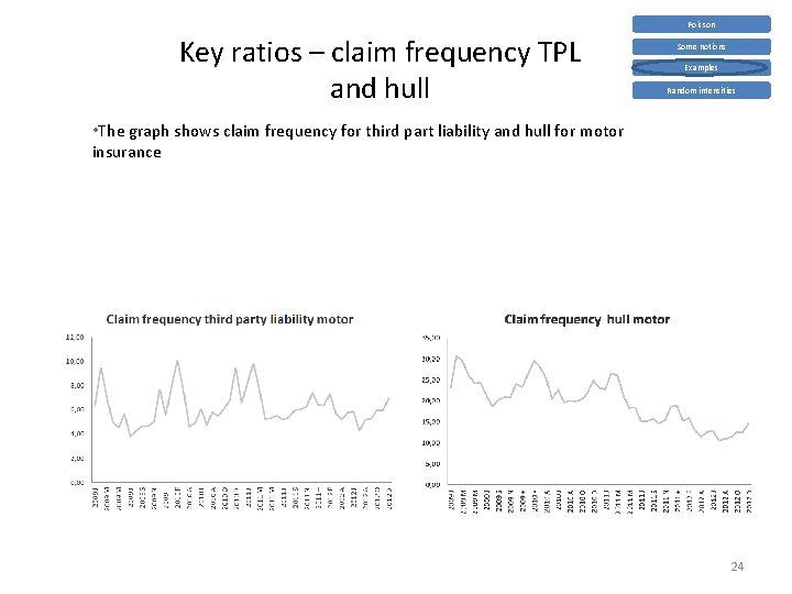
Poisson Key ratios – claim frequency TPL and hull Some notions Examples Random intensities • The graph shows claim frequency for third part liability and hull for motor insurance 24

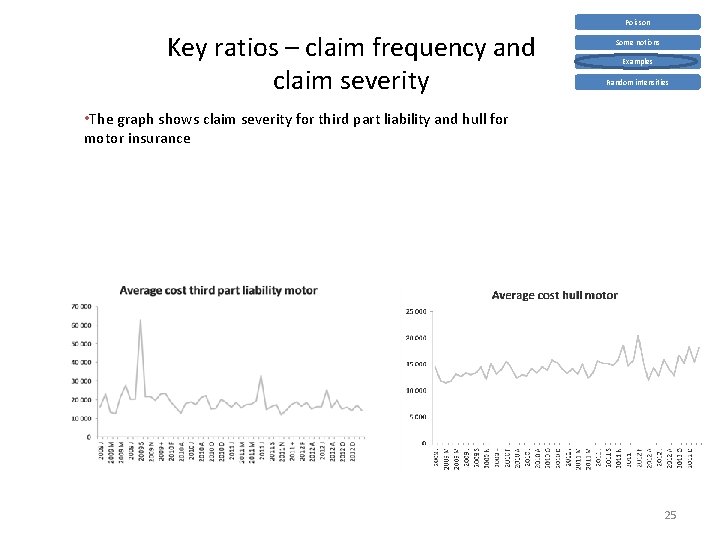
Poisson Key ratios – claim frequency and claim severity Some notions Examples Random intensities • The graph shows claim severity for third part liability and hull for motor insurance 25

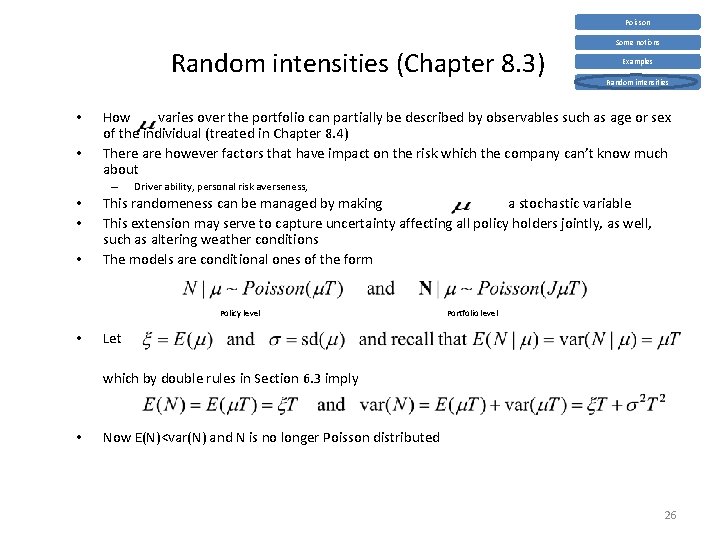
Poisson Random intensities (Chapter 8. 3) • • • Random intensities Driver ability, personal risk averseness, This randomeness can be managed by making a stochastic variable This extension may serve to capture uncertainty affecting all policy holders jointly, as well, such as altering weather conditions The models are conditional ones of the form Policy level • Examples How varies over the portfolio can partially be described by observables such as age or sex of the individual (treated in Chapter 8. 4) There are however factors that have impact on the risk which the company can’t know much about – • • Some notions Portfolio level Let which by double rules in Section 6. 3 imply • Now E(N)<var(N) and N is no longer Poisson distributed 26

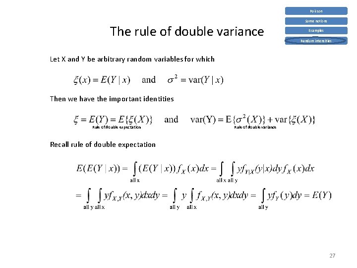
Poisson The rule of double variance Some notions Examples Random intensities Let X and Y be arbitrary random variables for which Then we have the important identities Rule of double expectation Rule of double variance Recall rule of double expectation 27

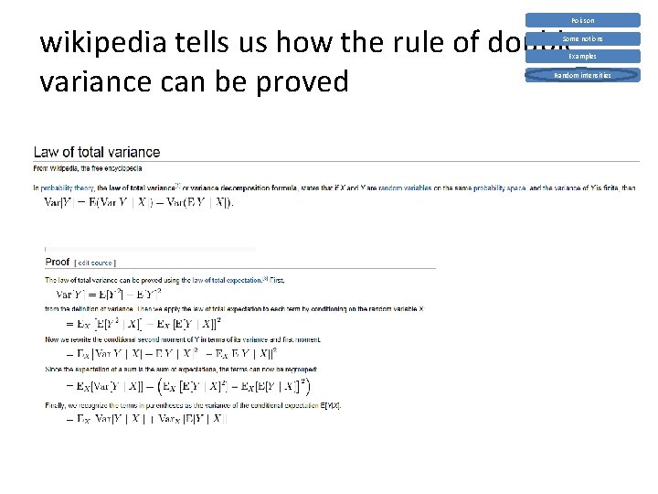
Poisson wikipedia tells us how the rule of double variance can be proved Some notions Examples Random intensities

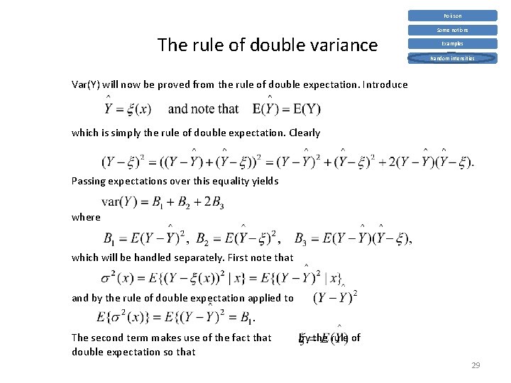
Poisson The rule of double variance Some notions Examples Random intensities Var(Y) will now be proved from the rule of double expectation. Introduce which is simply the rule of double expectation. Clearly Passing expectations over this equality yields where which will be handled separately. First note that and by the rule of double expectation applied to The second term makes use of the fact that double expectation so that by the rule of 29

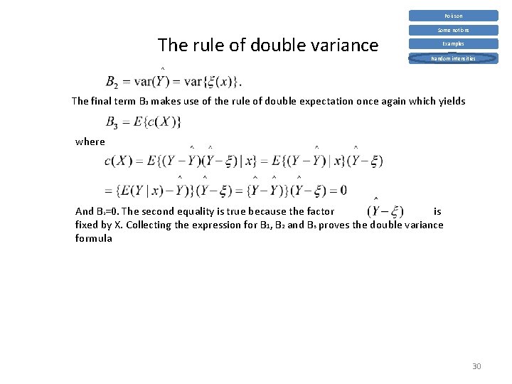
Poisson The rule of double variance Some notions Examples Random intensities The final term B 3 makes use of the rule of double expectation once again which yields where And B =0. The second equality is true because the factor is fixed by X. Collecting the expression for B 1, B 2 and B 3 proves the double variance formula 3 30

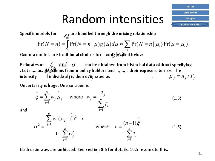
Poisson Random intensities Specific models for Some notions Examples Random intensities are handled through the mixing relationship Gamma models are traditional choices for and detailed below Estimates of can be obtained from historical data without specifying. Let n 1, . . . , nn be claims from n policy holders and T 1, . . . , TJ their exposure to risk. The intensity if individual j is then estimated as. Uncertainty is huge. One solution is (1. 5) and (1. 6) Both estimates are unbiased. See Section 8. 6 for details. 10. 5 returns to this. 31

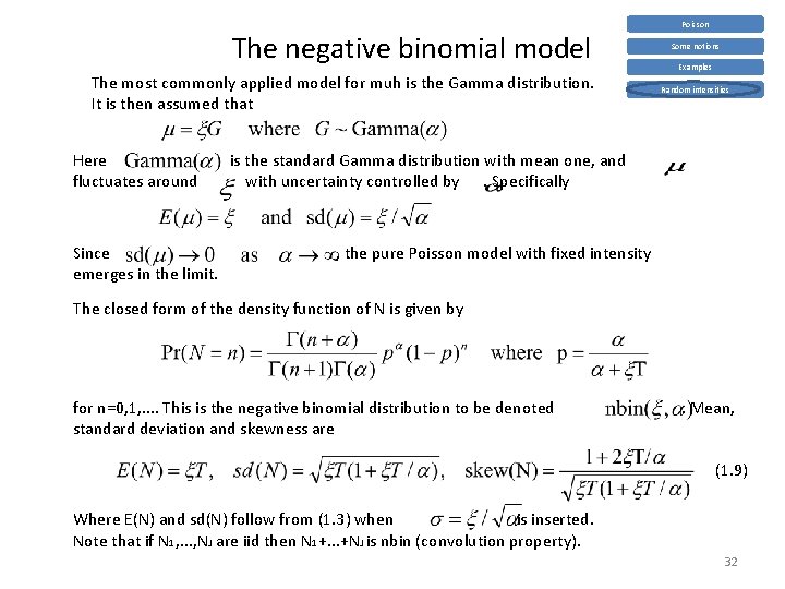
The negative binomial model The most commonly applied model for muh is the Gamma distribution. It is then assumed that Here fluctuates around Since emerges in the limit. Poisson Some notions Examples Random intensities is the standard Gamma distribution with mean one, and with uncertainty controlled by. Specifically , the pure Poisson model with fixed intensity The closed form of the density function of N is given by for n=0, 1, . . This is the negative binomial distribution to be denoted standard deviation and skewness are . Mean, (1. 9) Where E(N) and sd(N) follow from (1. 3) when is inserted. Note that if N 1, . . . , NJ are iid then N 1+. . . +NJ is nbin (convolution property). 32

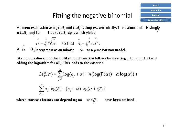
Poisson Fitting the negative binomial Some notions Examples Random intensities Moment estimation using (1. 5) and (1. 6) is simplest technically. The estimate of is simply in (1. 5), and for invoke (1. 8) right which yields If , interpret it as an infinite or a pure Poisson model. Likelihood estimation: the log likelihood function follows by inserting n j for n in (1. 9) and adding the logarithm for all j. This leads to the criterion where constant factors not depending on and have been omitted. 33