Reasons to review the linear model It is

Assumptions of Simple Linear Regression Unknown Relationship Y = b 0 + b 1

Assumptions (only necessary for inference)

The Method of Least Squares Data Assumption Total Squared “Error”

Explained versus Unexplained Variability * Y^ = b^0 + b^1 X Y 26

title "Height and FEV in 12 boys, 10 -15 years old"; data fev 1

proc sgplot data=fev 1 ht; scatter y=fev x=height; run;

title "Height and FEV in 12 boys, 10 -15 years old"; proc sgplot data=fev

proc reg data=fev 1 ht plots=none; model fev=height; quit;

proc reg data=fev 1 ht noprint outest=betas; model fev=height; quit; proc sql; select mean(fev)

data tmp (keep=totalssq modelssq errorssq); set fev 1 ht end=eod; fevhat=&a+&b*height; /*predicted FEV*/ fevresid=fev-fevhat;

Slides: 35

Download presentation

Reasons to review the linear model It is probably the most used and most easily understood statistical model. Understand it’s limitations for binary outcomes.

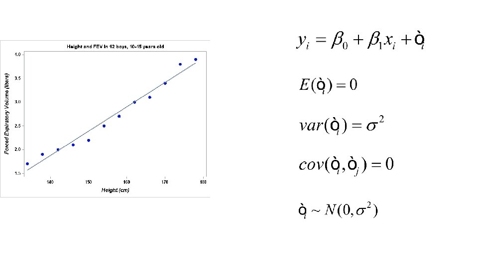
Assumptions of Simple Linear Regression Unknown Relationship Y = b 0 + b 1 X 4

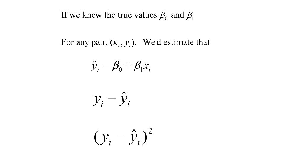
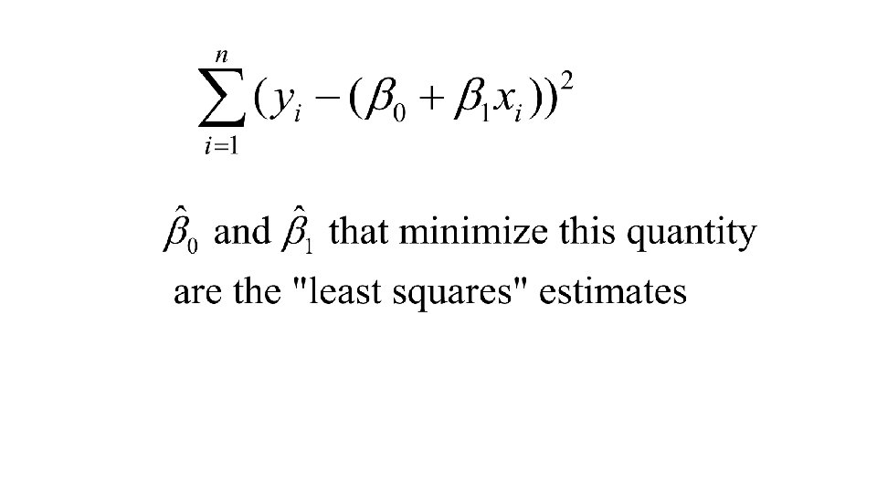
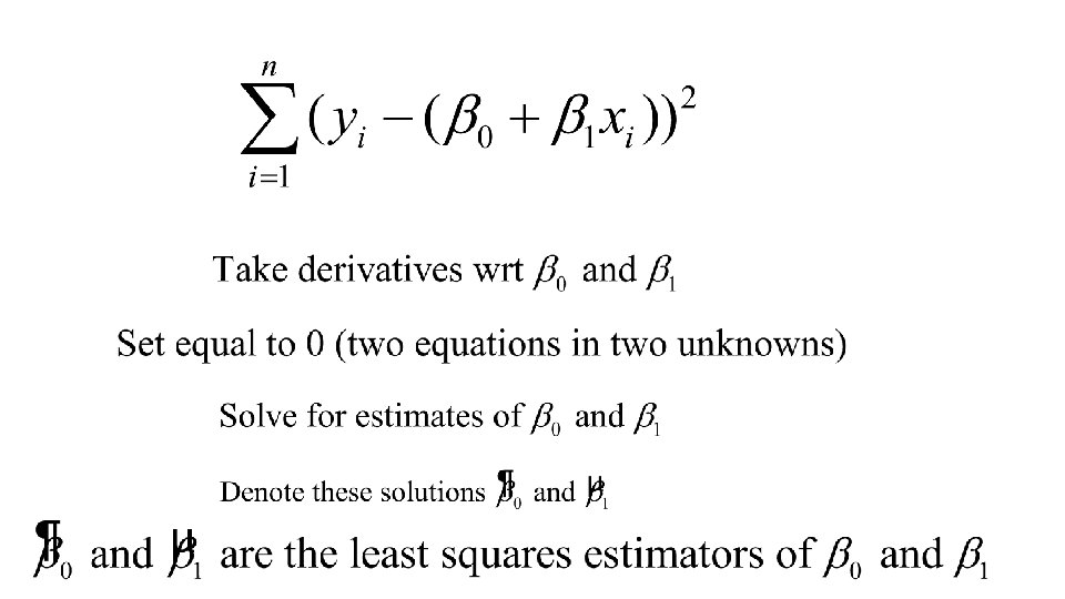
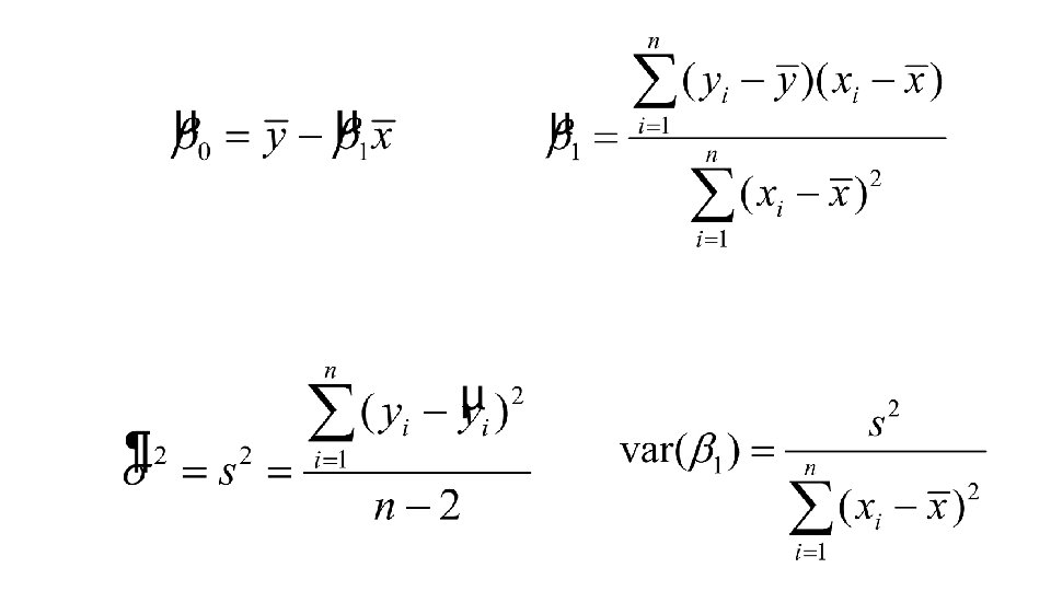
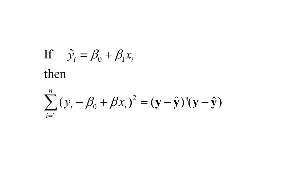
The Method of Least Squares

The equation of a straight line:

The Method of Least Squares

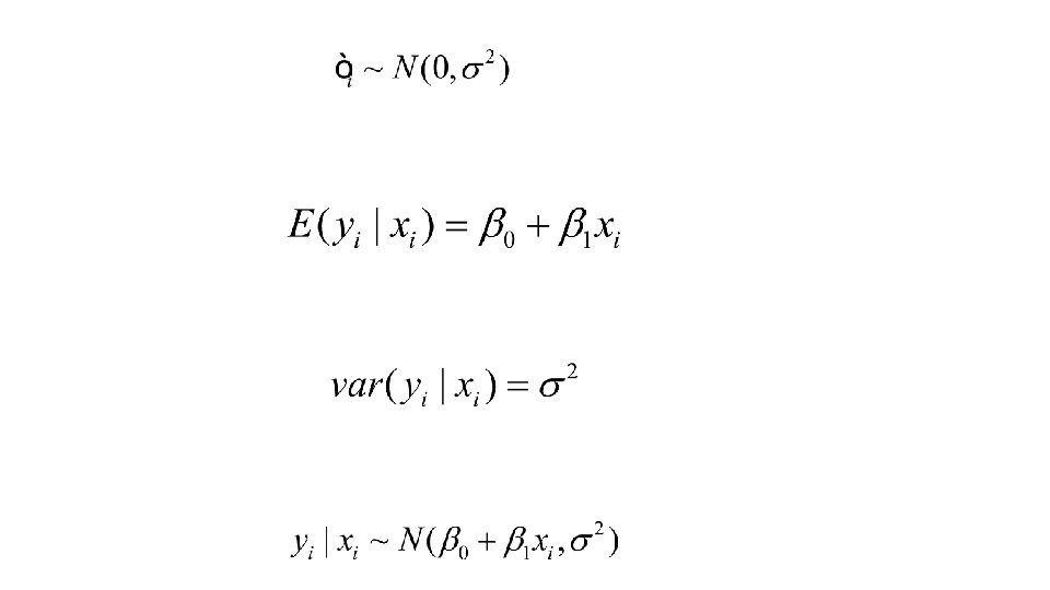
Assumptions (only necessary for inference)

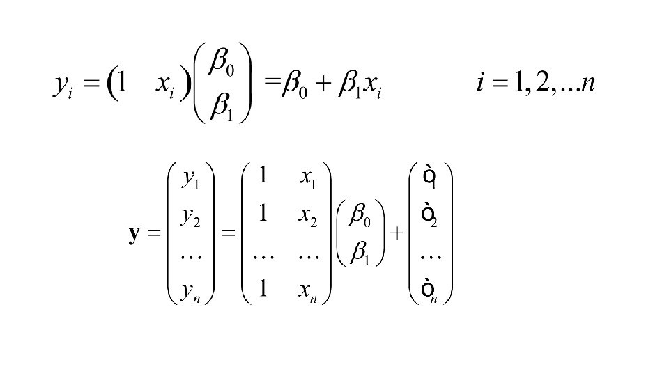
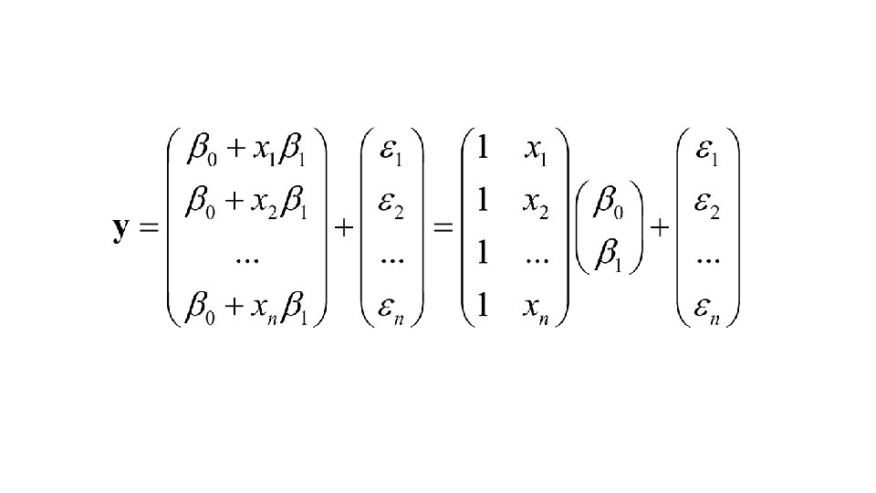
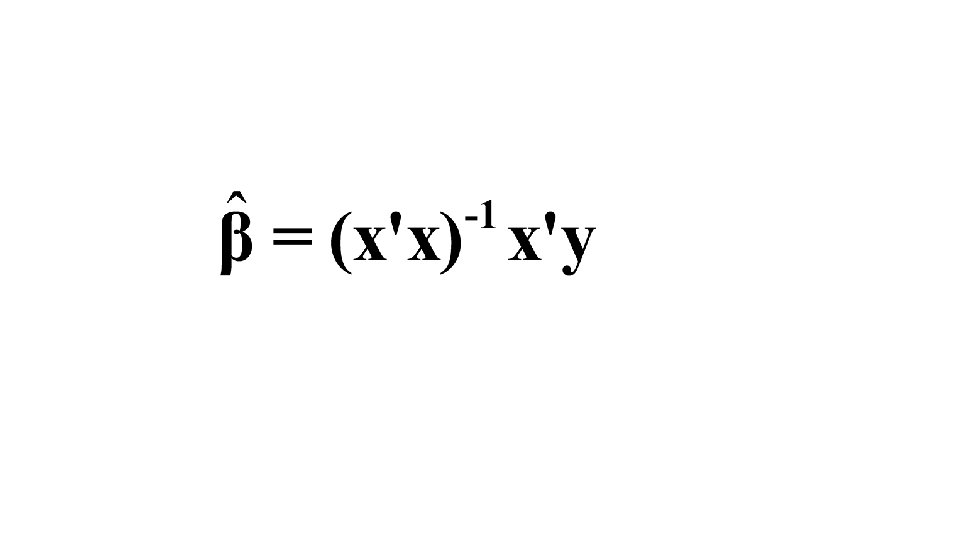
Vector/Matrix approach to least squares

The multivariate linear model.

The simple linear regression model.

The multiple linear regression model.

The Method of Least Squares Data Assumption Total Squared “Error”

A few statistical things 24

The Baseline (Null) Model Y 25

Explained versus Unexplained Variability * Y^ = b^0 + b^1 X Y 26

SST = SSR + SSE 27

Linear Regression with Proc Reg 28

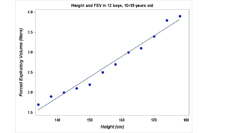
title "Height and FEV in 12 boys, 10 -15 years old"; data fev 1 ht; input height fev @@; label fev="Forced Expiratory Volume (liters)" height="Height (cm)"; datalines; 134 1. 7 158 2. 7 138 1. 9 162 3. 0 150 2. 2 142 2. 0 166 3. 1 146 2. 1 170 3. 4 154 2. 5 ; proc sql; select * from fev 1 ht order by height ; quit; title; 174 3. 8 178 3. 9

proc sgplot data=fev 1 ht; scatter y=fev x=height; run;

title "Height and FEV in 12 boys, 10 -15 years old"; proc sgplot data=fev 1 ht; scatter y=fev x=height/ markerattrs=(color=blue symbol=Circle. Filled size=10); reg y=fev x=height; xaxis LABELATTRS=(Color=Black Family=Arial Size=12 Style=Italic Weight=Bold) valueattrs=(size=10 pt weight=bold); yaxis LABELATTRS=(Color=Black Family=Arial Size=12 Style=Italic Weight=Bold) valueattrs=(size=10 pt weight=bold); run; title;

proc reg data=fev 1 ht plots=none; model fev=height; quit;

proc reg data=fev 1 ht noprint outest=betas; model fev=height; quit; proc sql; select mean(fev) into : mnfev from fev 1 ht; select intercept, height into : a, : b from betas; quit; %put &mnfev &a &b; 34

data tmp (keep=totalssq modelssq errorssq); set fev 1 ht end=eod; fevhat=&a+&b*height; /*predicted FEV*/ fevresid=fev-fevhat; /* residual FEV*/ residsq=fevresid**2; errorssq+residsq; totalssq+(fev-&mnfev)**2; if eod then do; modelssq=totalssq-errorssq; output; Aend; run; proc print data=tmp; run; 35