RealTime Template Tracking Stefan Holzer Computer Aided Medical

Real-Time Template Tracking Stefan Holzer Computer Aided Medical Procedures (CAMP), Technische Universität München, Germany

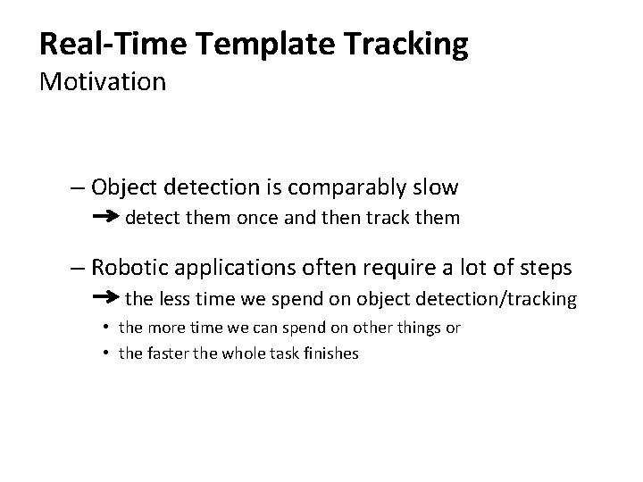
Real-Time Template Tracking Motivation – Object detection is comparably slow detect them once and then track them – Robotic applications often require a lot of steps the less time we spend on object detection/tracking • the more time we can spend on other things or • the faster the whole task finishes

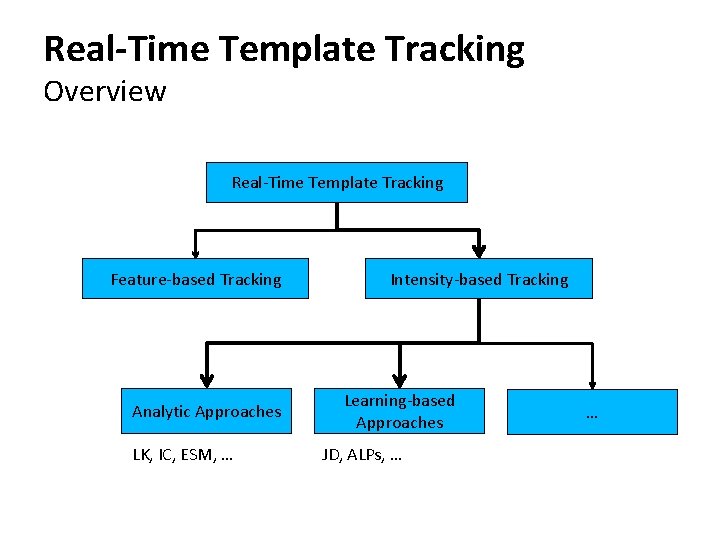
Real-Time Template Tracking Overview Real-Time Template Tracking Feature-based Tracking Analytic Approaches LK, IC, ESM, … Intensity-based Tracking Learning-based Approaches JD, ALPs, … …

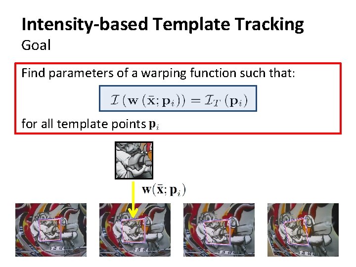
Intensity-based Template Tracking Goal Find parameters of a warping function such that: for all template points

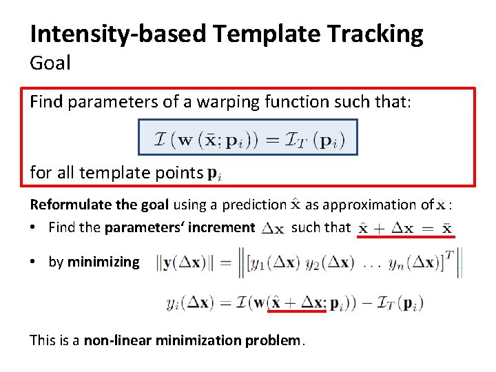
Intensity-based Template Tracking Goal Find parameters of a warping function such that: for all template points Reformulate the goal using a prediction as approximation of : • Find the parameters‘ increment such that • by minimizing This is a non-linear minimization problem.

Intensity-based Template Tracking Lukas-Kanade Uses the Gauss-Newton method for minimization: • Applies a first-order Taylor series approximation • Minimizes iteratively B. D. Lucas and T. Kanade. An iterative image registration technique with an application to stereo vision, 1981.

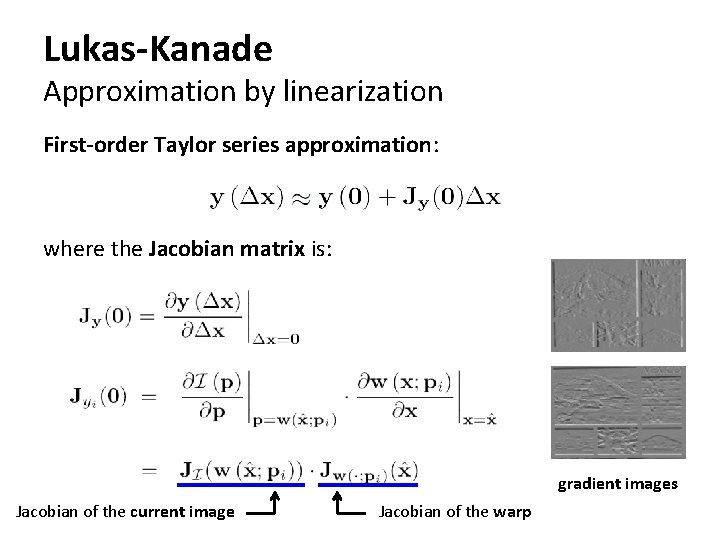
Lukas-Kanade Approximation by linearization First-order Taylor series approximation: where the Jacobian matrix is: gradient images Jacobian of the current image Jacobian of the warp

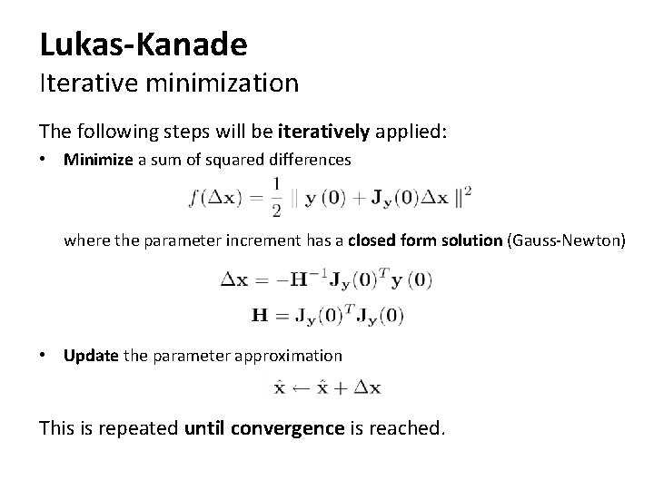
Lukas-Kanade Iterative minimization The following steps will be iteratively applied: • Minimize a sum of squared differences where the parameter increment has a closed form solution (Gauss-Newton) • Update the parameter approximation This is repeated until convergence is reached.

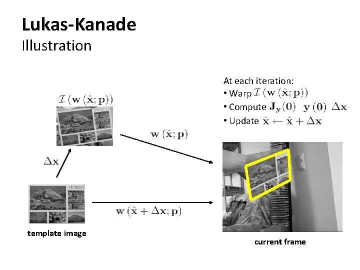
Lukas-Kanade Illustration At each iteration: • Warp • Compute • Update template image current frame

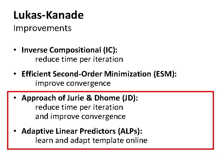
Lukas-Kanade Improvements • Inverse Compositional (IC): reduce time per iteration • Efficient Second-Order Minimization (ESM): improve convergence • Approach of Jurie & Dhome (JD): reduce time per iteration and improve convergence • Adaptive Linear Predictors (ALPs): learn and adapt template online

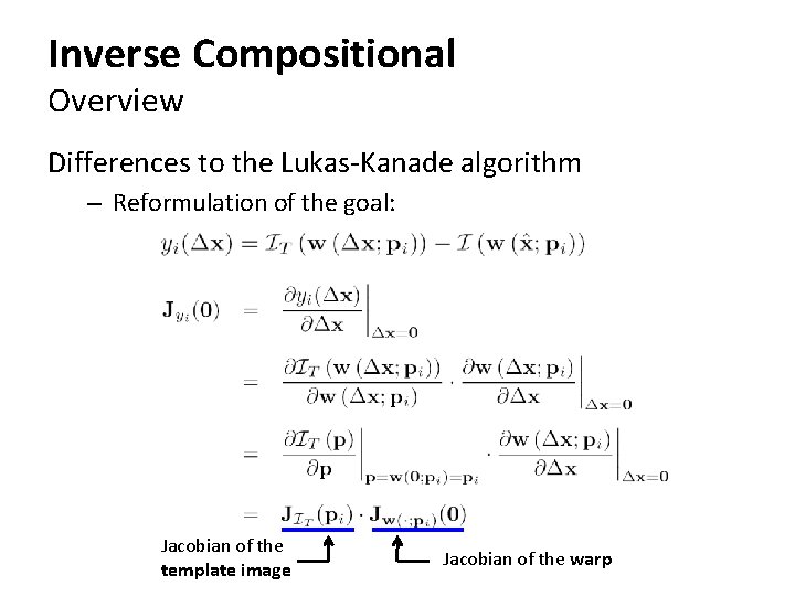
Inverse Compositional Overview Differences to the Lukas-Kanade algorithm – Reformulation of the goal: Jacobian of the template image Jacobian of the warp

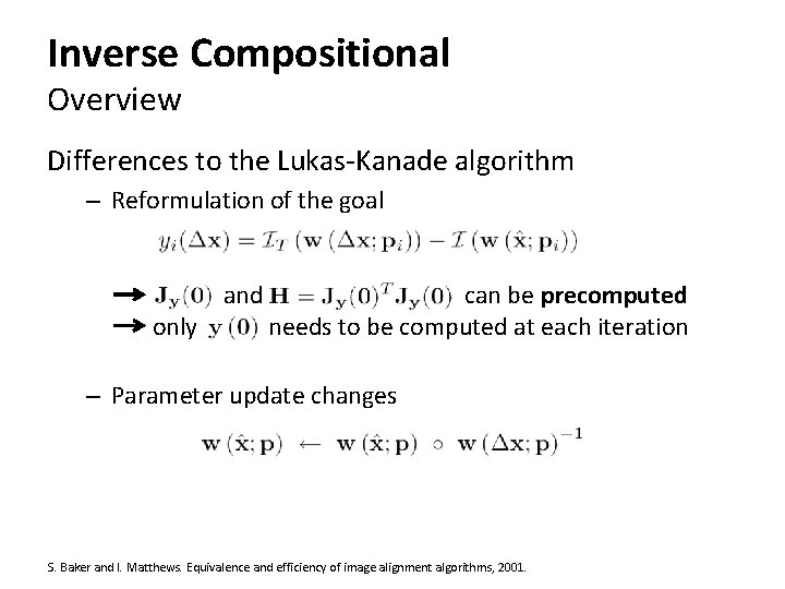
Inverse Compositional Overview Differences to the Lukas-Kanade algorithm – Reformulation of the goal only and can be precomputed needs to be computed at each iteration – Parameter update changes S. Baker and I. Matthews. Equivalence and efficiency of image alignment algorithms, 2001.

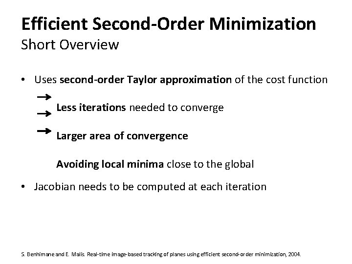
Efficient Second-Order Minimization Short Overview • Uses second-order Taylor approximation of the cost function Less iterations needed to converge Larger area of convergence Avoiding local minima close to the global • Jacobian needs to be computed at each iteration S. Benhimane and E. Malis. Real-time image-based tracking of planes using efficient second-order minimization, 2004.

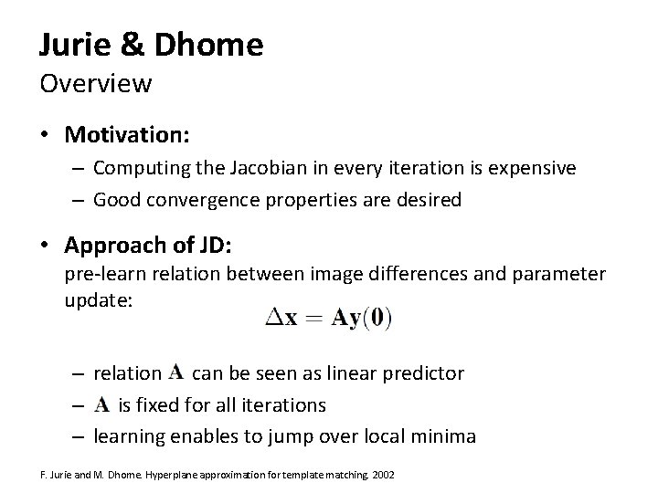
Jurie & Dhome Overview • Motivation: – Computing the Jacobian in every iteration is expensive – Good convergence properties are desired • Approach of JD: pre-learn relation between image differences and parameter update: – relation can be seen as linear predictor – is fixed for all iterations – learning enables to jump over local minima F. Jurie and M. Dhome. Hyperplane approximation for template matching. 2002

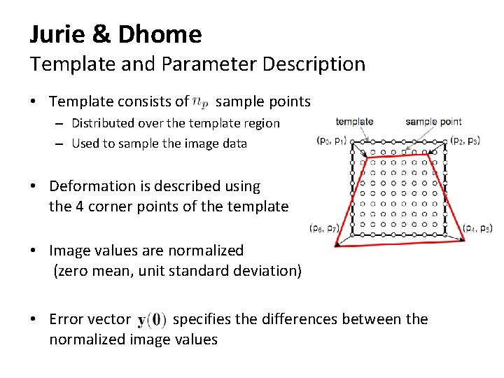
Jurie & Dhome Template and Parameter Description • Template consists of sample points – Distributed over the template region – Used to sample the image data • Deformation is described using the 4 corner points of the template • Image values are normalized (zero mean, unit standard deviation) • Error vector specifies the differences between the normalized image values

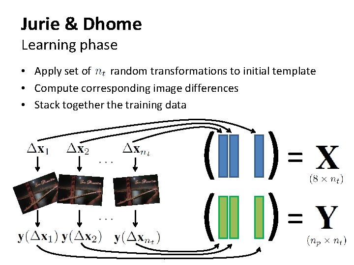
Jurie & Dhome Learning phase • Apply set of random transformations to initial template • Compute corresponding image differences • Stack together the training data ( )=

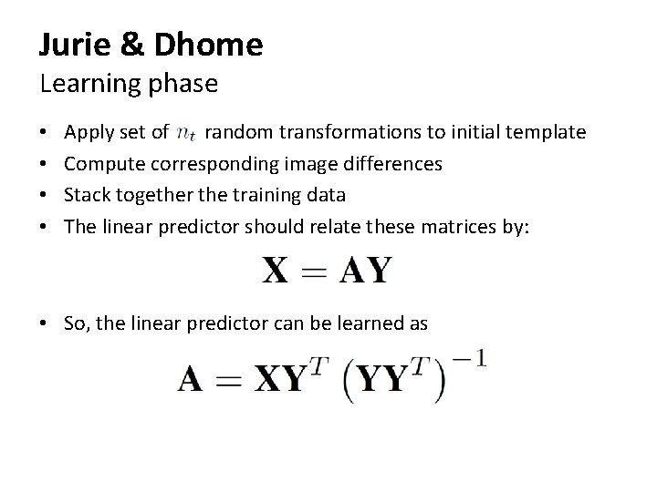
Jurie & Dhome Learning phase • • Apply set of random transformations to initial template Compute corresponding image differences Stack together the training data The linear predictor should relate these matrices by: • So, the linear predictor can be learned as

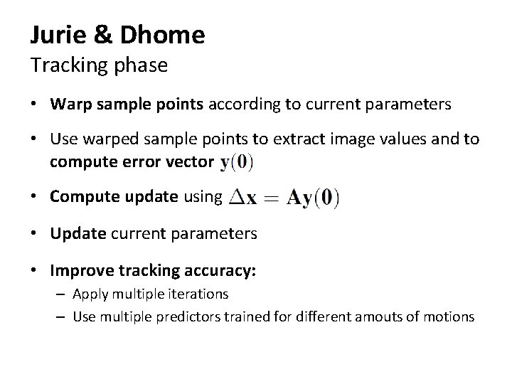
Jurie & Dhome Tracking phase • Warp sample points according to current parameters • Use warped sample points to extract image values and to compute error vector • Compute update using • Update current parameters • Improve tracking accuracy: – Apply multiple iterations – Use multiple predictors trained for different amouts of motions

Jurie & Dhome Limitations • Learning large templates is expensive not possible online • Shape of template cannot be adapted template has to be relearned after each modification • Tracking accuracy is inferior to LK, IC, … use JD as initialization for one of those

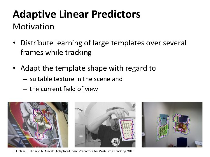
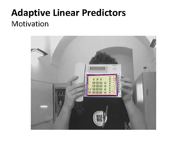
Adaptive Linear Predictors Motivation • Distribute learning of large templates over several frames while tracking • Adapt the template shape with regard to – suitable texture in the scene and – the current field of view S. Holzer, S. Ilic and N. Navab. Adaptive Linear Predictors for Real-Time Tracking, 2010.

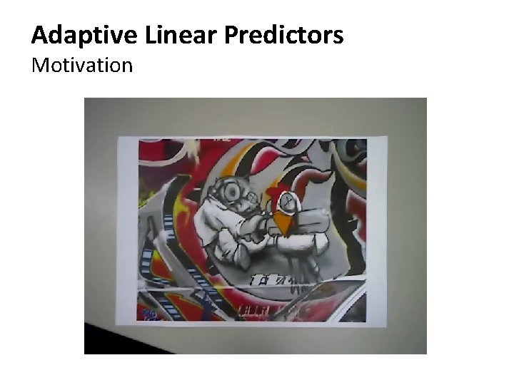
Adaptive Linear Predictors Motivation

Adaptive Linear Predictors Motivation

Adaptive Linear Predictors Motivation

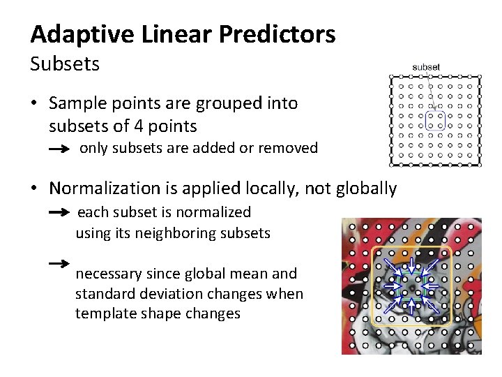
Adaptive Linear Predictors Subsets • Sample points are grouped into subsets of 4 points only subsets are added or removed • Normalization is applied locally, not globally each subset is normalized using its neighboring subsets necessary since global mean and standard deviation changes when template shape changes

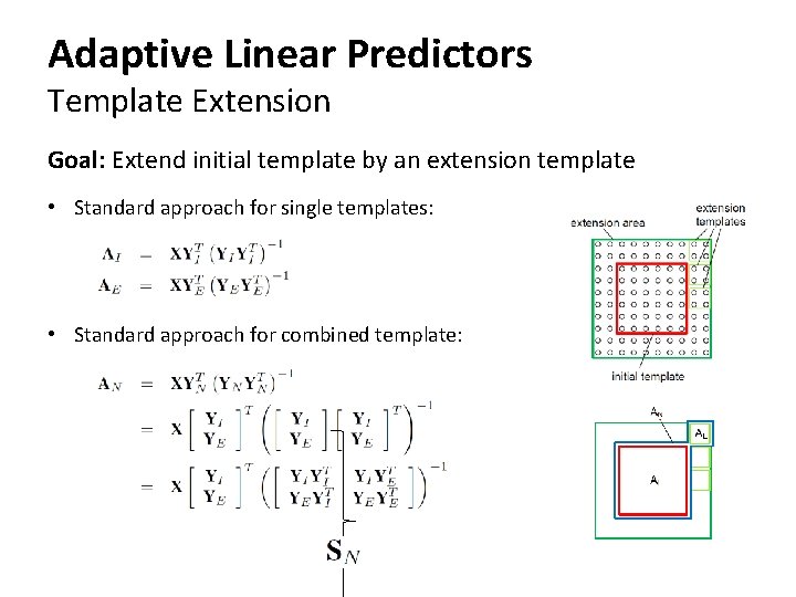
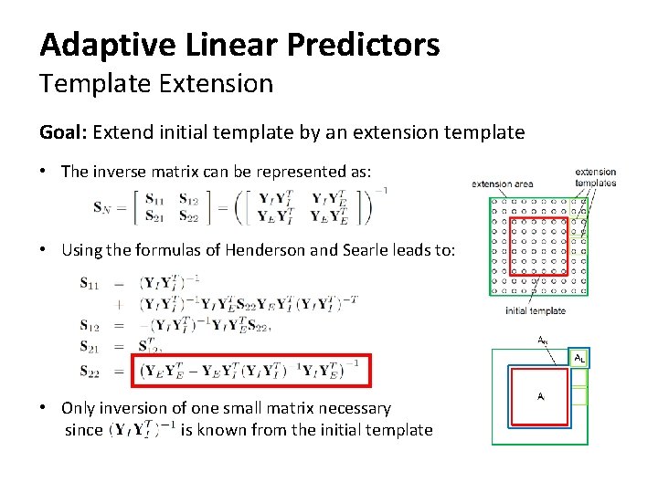
Adaptive Linear Predictors Template Extension Goal: Extend initial template by an extension template • Standard approach for single templates: • Standard approach for combined template:

Adaptive Linear Predictors Template Extension Goal: Extend initial template by an extension template • The inverse matrix can be represented as: • Using the formulas of Henderson and Searle leads to: • Only inversion of one small matrix necessary since is known from the initial template

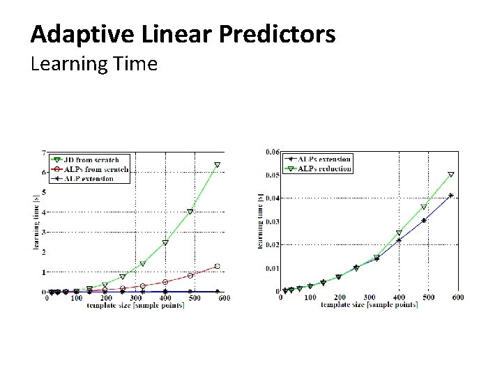
Adaptive Linear Predictors Learning Time

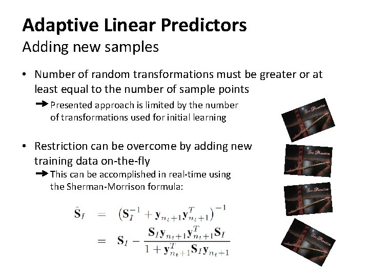
Adaptive Linear Predictors Adding new samples • Number of random transformations must be greater or at least equal to the number of sample points Presented approach is limited by the number of transformations used for initial learning • Restriction can be overcome by adding new training data on-the-fly This can be accomplished in real-time using the Sherman-Morrison formula:

Thank you for your attention! Questions?