Realignment SPM 5 Methods for Dummies 2007 P

Realignment SPM 5 - Methods for Dummies 2007 P. Schwingenschuh

Spatial Registration We use spatial registration to align images: Ø Realigning and unwarping • Motion correction (realignment) adjusts for an individuals head movements → creates a spatially stabilized image • But residual errors…. . → unwarping Ø Co-registration aligns two images of different modalities from the same individual. Ø Spatial Normalization aligns images from

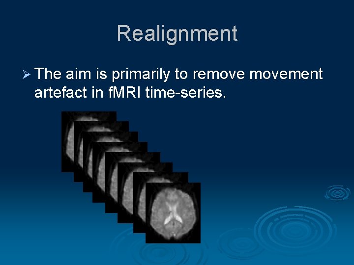
Realignment Ø The aim is primarily to removement artefact in f. MRI time-series.

Reasons for Motion Correction Ø Subjects will always move in the scanner Ø The sensitivity of the analysis depends on the residual noise in the image series, so movement that is unrelated to the subject’s task will add to this noise and hence realignment will increase the sensitivity Ø However, subject movement may also correlate with the task… Ø …in which case realignment may reduce sensitivity (and it may not be possible to discount artefacts that owe to motion)

Realign Ø SPM 5 l l l manual: This routine realigns a time-series of images acquired from the same subject using a least squares approach and a 6 parameter (rigid body) spatial transformation. The first image in the list specified by the user is used as a reference to which all subsequent scans are realigned. The reference scan does not have to the first chronologically and it may be wise to chose a ”representative scan” in this role.

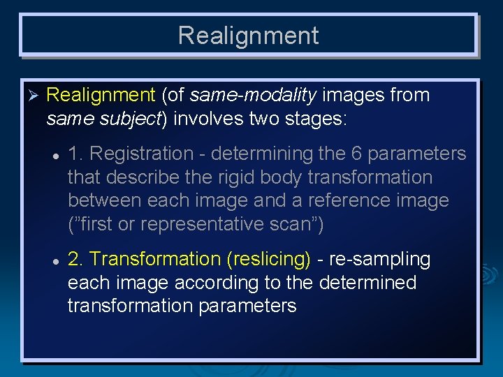
Realignment-2 steps Ø Realignment (of same-modality images from same subject) involves two stages: l l 1. Registration - determining the 6 parameters that describe the rigid body transformation between each source image and a reference image (in f. MRI first or representative scan) 2. Transformation (reslicing) - re-sampling each image according to the determined transformation parameters

Motion Correction Ø Motion crucial: l l Correction (‘Realignment’) is We want to compare same part of the brain across time. If we do not MC, there will be a lot of variability in our data. Ø Mathematically, l l We assume that all images show the same brain, so rigid body transform is sufficient. All images have the same contrast.

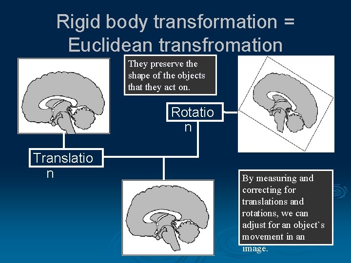
Rigid body transformation = Euclidean transfromation They preserve the shape of the objects that they act on. Rotatio n Translatio n By measuring and correcting for translations and rotations, we can adjust for an object`s movement in an image.

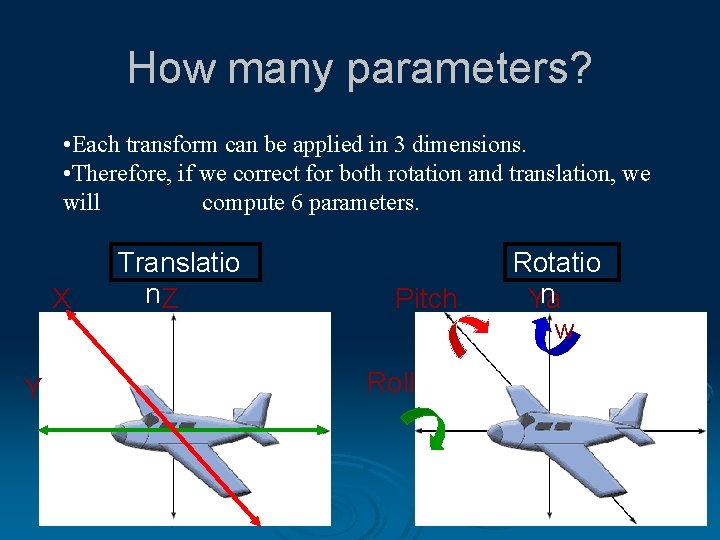
How many parameters? • Each transform can be applied in 3 dimensions. • Therefore, if we correct for both rotation and translation, we will compute 6 parameters. X Y Translatio n. Z Pitch Roll Rotatio n Ya w

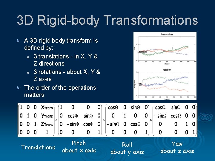
3 D Rigid-body Transformations A 3 D rigid body transform is defined by: l 3 translations - in X, Y & Z directions l 3 rotations - about X, Y & Z axes Ø The order of the operations matters Ø Translations Pitch about x axis Roll about y axis Yaw about z axis

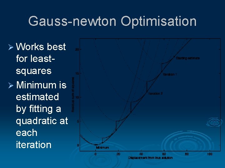
Gauss-newton Optimisation Ø Works best for leastsquares Ø Minimum is estimated by fitting a quadratic at each iteration

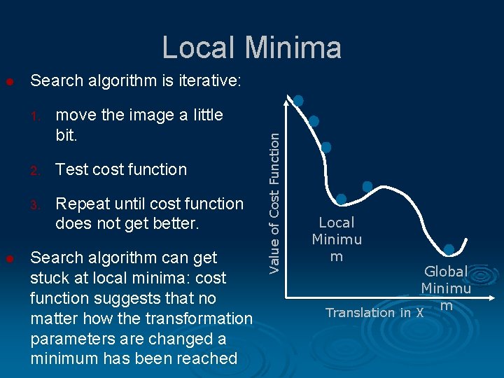
Local Minima l Search algorithm is iterative: 1. move the image a little bit. 2. Test cost function 3. Repeat until cost function does not get better. Search algorithm can get stuck at local minima: cost function suggests that no matter how the transformation parameters are changed a minimum has been reached Value of Cost Function l Local Minimu m Global Minimu m Translation in X

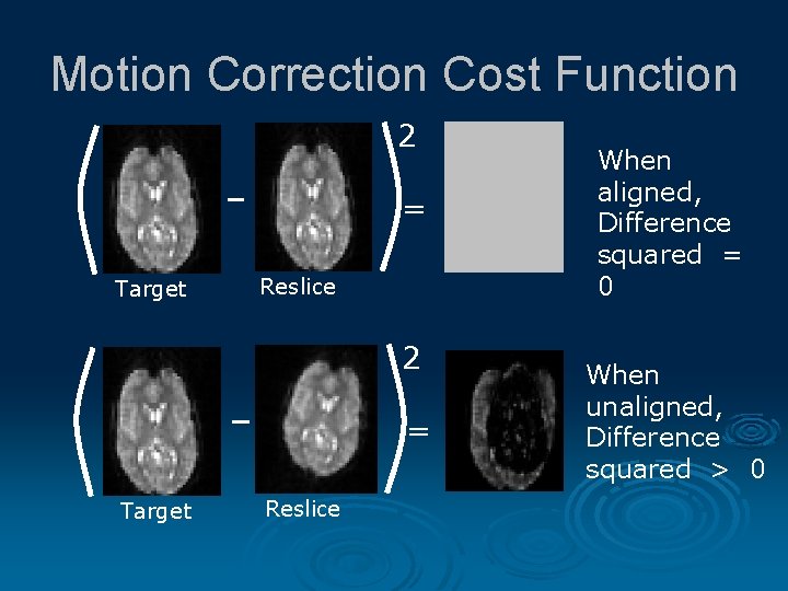
Motion Correction Cost Function 2 = Target Reslice When aligned, Difference squared = 0 When unaligned, Difference squared > 0

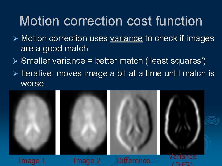
Motion correction cost function Motion correction uses variance to check if images are a good match. Ø Smaller variance = better match (‘least squares’) Ø Iterative: moves image a bit at a time until match is worse. Ø Image 1 Image 2 Difference Variance

Realignment Ø Realignment (of same-modality images from same subject) involves two stages: l l 1. Registration - determining the 6 parameters that describe the rigid body transformation between each image and a reference image (”first or representative scan”) 2. Transformation (reslicing) - re-sampling each image according to the determined transformation parameters

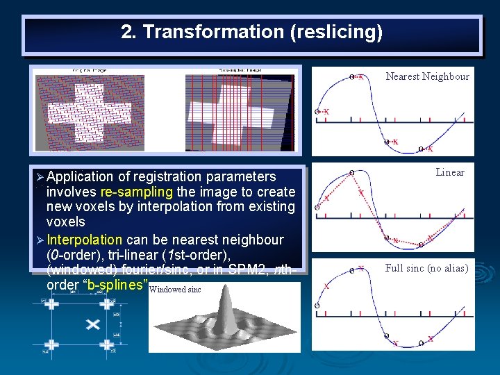
Transformation The intensity of each voxel in the transformed image must be determined from the intensities in the original image. Ø In order to realign images with subvoxel accuracy, the spatial transformations will involve fractions of a voxel. Ø It is therefore necessary to resample the image at positions between the centers of voxels. Ø This requires an interpolation scheme to estimate the intensity of a voxel, based on the intensity of its neighbours. Ø

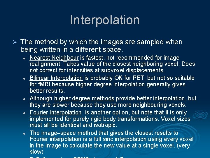
Interpolation Ø The method by which the images are sampled when being written in a different space. l l l Nearest Neighbour is fastest, not recommended for image realignment. Takes value of the closest neighboring voxel. Does not correct for intensities at subvoxel displacements. Bilinear Interpolation is probably OK for PET, but not so suitable for f. MRI because higher degree interpolation generally gives better results. Although higher degree methods provide better interpolation, but they are slower because they use more neighbouring voxels. Fourier Interpolation is another option, but note that it is only implemented for purely rigid body transformations. Voxel sizes must all be identical and isotropic. The image–space method that gives the closest results to Fourier interpolation is a full sinc interpolation using every voxel in the image to calculate the new value at a single voxel. (very slow)

2. Transformation (reslicing) Nearest Neighbour Ø Application of registration parameters involves re-sampling the image to create new voxels by interpolation from existing voxels Ø Interpolation can be nearest neighbour (0 -order), tri-linear (1 st-order), (windowed) fourier/sinc, or in SPM 2, nthorder “b-splines” Windowed sinc Linear Full sinc (no alias)

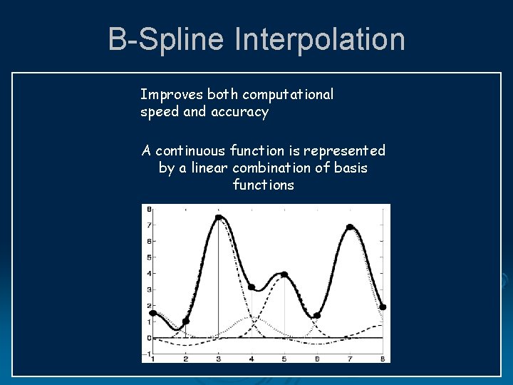
B-Spline Interpolation Improves both computational speed and accuracy A continuous function is represented by a linear combination of basis functions

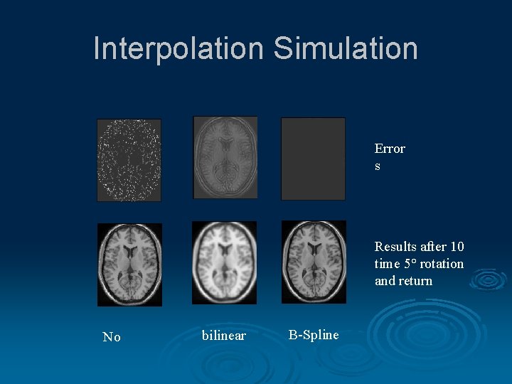
Interpolation Simulation Error s Results after 10 time 5° rotation and return No bilinear B-Spline

Residual Errors after Realignment Ø Interpolation errors, especially with tri-linear interpolation and small-window sinc Ø Ghosts (and other artefacts) in the image (which do not move as a rigid body) Ø Rapid movements within a scan (which cause nonrigid image deformation) Ø Spin excitation history effects (residual magnetisation effects of previous scans) Ø Interaction between movement and local field inhomogeniety, giving non-rigid distortion →

Sources & References & So On… Ø SPM for Dummies 2006 Ø Rik Henson’s SPM minicourse Ø John Ashburner’s lecture on spatial preprocessing (SPM course USA 2005) Ø Human Brain Function, 2 nd Edition (Edited by J Ashburner, K Friston, W Penny) – mostly chapter 2. Ø SPM 5 manual

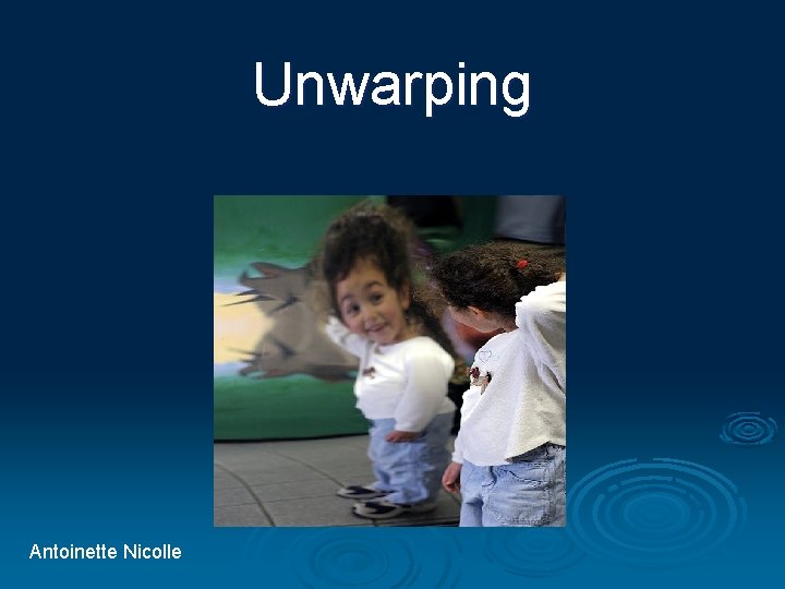
Unwarping Antoinette Nicolle

Pre-processing steps Ø Voxel-based analysis assumes that the data from a particular voxel all derive from the same part of the brain Ø So, for within-subject and between-subject comparisons we need: l l l Slice time correction Realignment to ‘undo’ the effects of subject motion Co-registration Normalisation Smoothing

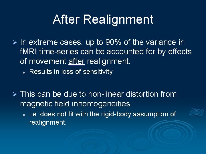
After Realignment Ø In extreme cases, up to 90% of the variance in f. MRI time-series can be accounted for by effects of movement after realignment. l Ø Results in loss of sensitivity This can be due to non-linear distortion from magnetic field inhomogeneities l i. e. does not fit with the rigid-body assumption of realignment.

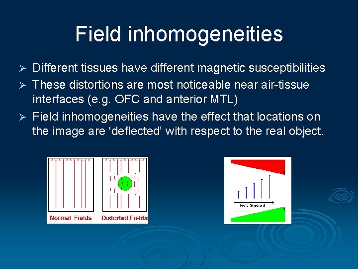
Field inhomogeneities Different tissues have different magnetic susceptibilities Ø These distortions are most noticeable near air-tissue interfaces (e. g. OFC and anterior MTL) Ø Field inhomogeneities have the effect that locations on the image are ‘deflected’ with respect to the real object. Ø

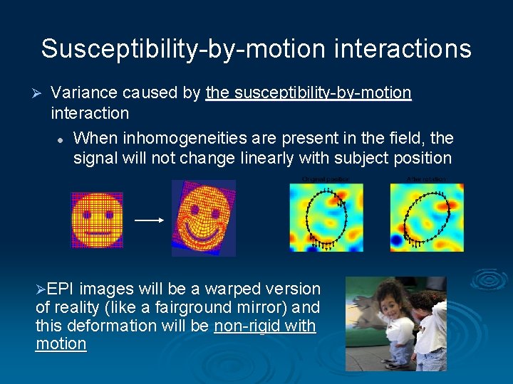
Susceptibility-by-motion interactions Ø Variance caused by the susceptibility-by-motion interaction l When inhomogeneities are present in the field, the signal will not change linearly with subject position ØEPI images will be a warped version of reality (like a fairground mirror) and this deformation will be non-rigid with motion

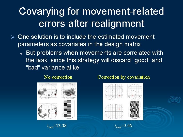
Covarying for movement-related errors after realignment Ø One solution is to include the estimated movement parameters as covariates in the design matrix l But problems when movements are correlated with the task, since this strategy will discard “good” and “bad” variance alike No correction tmax=13. 38 Correction by covariation tmax=5. 06

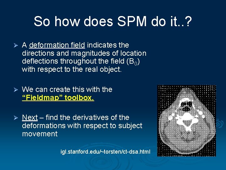
So how does SPM do it. . ? Ø A deformation field indicates the directions and magnitudes of location deflections throughout the field (B 0) with respect to the real object. Ø We can create this with the “Fieldmap” toolbox. Ø Next – find the derivatives of the deformations with respect to subject movement igl. stanford. edu/~torsten/ct-dsa. html

The susceptibility-by-motion interaction In practice, rather than generating a statistical field map for every image in the EPI data set, we compute how one map is warped over subsequent scans. Ø Computing how the images are warped over subsequent scans requires knowing how the deformation fields change with displacement of the subject, i. e. the derivatives of deformation with respect to subject motion. Ø UNWARP attempts to do this and then re-samples the voxels accordingly

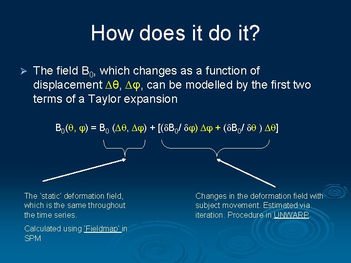
How does it do it? Ø The field B 0, which changes as a function of displacement ∆θ, ∆φ, can be modelled by the first two terms of a Taylor expansion B 0( , ) = B 0 ( , ) + [(δB 0/ δ ) + (δB 0/ δ ) ] ( The ‘static’ deformation field, which is the same throughout the time series. Calculated using ‘Fieldmap’ in SPM Changes in the deformation field with subject movement. Estimated via iteration. Procedure in UNWARP.

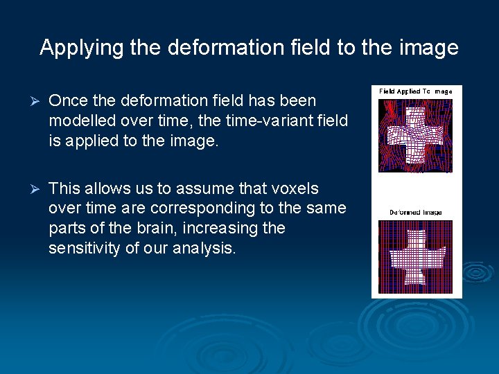
Applying the deformation field to the image Ø Once the deformation field has been modelled over time, the time-variant field is applied to the image. Ø This allows us to assume that voxels over time are corresponding to the same parts of the brain, increasing the sensitivity of our analysis.

In practice… Subject movements are quite small Ø With the latest scanners, distortions are typically quite small, and distortion-bymotion interactions even smaller Ø Small distortions result from: Ø a) b) c) Fast gradients Low field (i. e. <3 T) Low resolution (smoothing)

Assumptions of Unwarp Ø That the susceptibility-by-motion interaction is responsible for a sizeable part of the residual movement-related variance. But: l l l Ø Subject movement between slice acquisition (slice-to-vol effects) Susceptibility-dropout-by-motion interaction Spin-history effects Note also that the deformation field does not give us the “true” version of the time-series, but rather a level of average distortion.

References http: //www. fil. ion. ucl. ac. uk/spm/toolbox/unwarp/ Ø Slides by Mary Summers (Mf. D 2006) Ø John Ashburner’s slides http: //www. fil. ion. ucl. ac. uk/spm/course/#slides Ø Andersson JLR, Hutton C, Ashburner J, Turner R, Friston K (2001) Modelling geometric deformations in EPI time series. Neuroimage 13: 903 -919 Ø http: //www. cis. rit. edu/htbooks/mri/index. html (J Hornak’s tutorial) Ø