Readings Chapter 4 Linear Programming Applications in Marketing

Readings Chapter 4 Linear Programming Applications in Marketing, Finance, and Operations Management BA 452 Lesson A. 9 Operations Management Applications 1

Overview BA 452 Lesson A. 9 Operations Management Applications 2

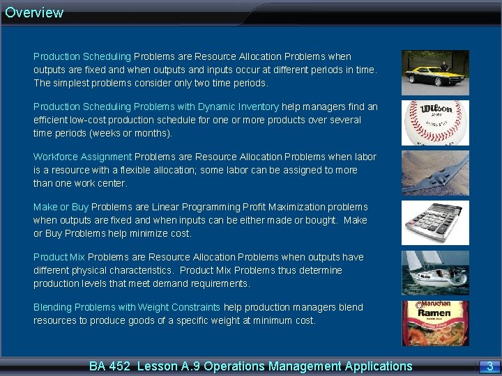
Overview Production Scheduling Problems are Resource Allocation Problems when outputs are fixed and when outputs and inputs occur at different periods in time. The simplest problems consider only two time periods. Production Scheduling Problems with Dynamic Inventory help managers find an efficient low-cost production schedule for one or more products over several time periods (weeks or months). Workforce Assignment Problems are Resource Allocation Problems when labor is a resource with a flexible allocation; some labor can be assigned to more than one work center. Make or Buy Problems are Linear Programming Profit Maximization problems when outputs are fixed and when inputs can be either made or bought. Make or Buy Problems help minimize cost. Product Mix Problems are Resource Allocation Problems when outputs have different physical characteristics. Product Mix Problems thus determine production levels that meet demand requirements. Blending Problems with Weight Constraints help production managers blend resources to produce goods of a specific weight at minimum cost. BA 452 Lesson A. 9 Operations Management Applications 3

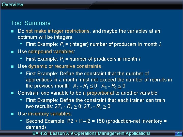
Overview Tool Summary n n n Do not make integer restrictions, and maybe the variables at an optimum will be integers. • First Example: Pi = (integer) number of producers in month i. Use compound variables: • First Example: Pi = number of producers in month i Use dynamic or recursive constraints: • First Example: Define the constraint that the number of apprentices in a month must not exceed the number of recruits in the previous month: A 2 - R 1 < 0; A 3 - R 2 < 0 Constrain one variable to be a proportional to another variable: • First Example: Define the constraint that each trainer can train two recruits: 2 T 1 - R 1 > 0; 2 T 2 - R 2 > 0 Use inventory variables: • Second Example: P 2 + I 1–I 2 = 150 (production-net inventory = demand) BA 452 Lesson A. 9 Operations Management Applications 4

Production Scheduling BA 452 Lesson A. 9 Operations Management Applications 5

Production Scheduling Overview Production Scheduling Problems are Resource Allocation Problems when outputs are fixed and when outputs and inputs occur at different periods in time. Production Scheduling Problems thus help managers find an efficient low-cost production schedule for one or more products over several periods in the future (weeks or months). The manager determines the production levels that meet demand requirements, given limitations on production capacity, labor capacity, and storage space, while minimizing total production and storage costs. The simplest problems consider only two time periods. BA 452 Lesson A. 9 Operations Management Applications 6

Production Scheduling Question: Chip Foose is the owner of Chip Foose Custom Cars. Chip has just received orders for 1, 000 standard wheels and 1, 250 deluxe wheels next month and for 800 standard and 1, 500 deluxe the following month. All orders must be filled. The cost of making standard wheels is $10 and deluxe wheels is $16. Overtime rates are 50% higher. There are 1, 000 hours of regular time and 500 hours of overtime available each month. It takes. 5 hour to make a standard wheel and. 6 hour to make a deluxe wheel. The cost of storing a wheel from one month to the next is $2. Minimize total production and inventory costs for standard and deluxe wheels. BA 452 Lesson A. 9 Operations Management Applications 7

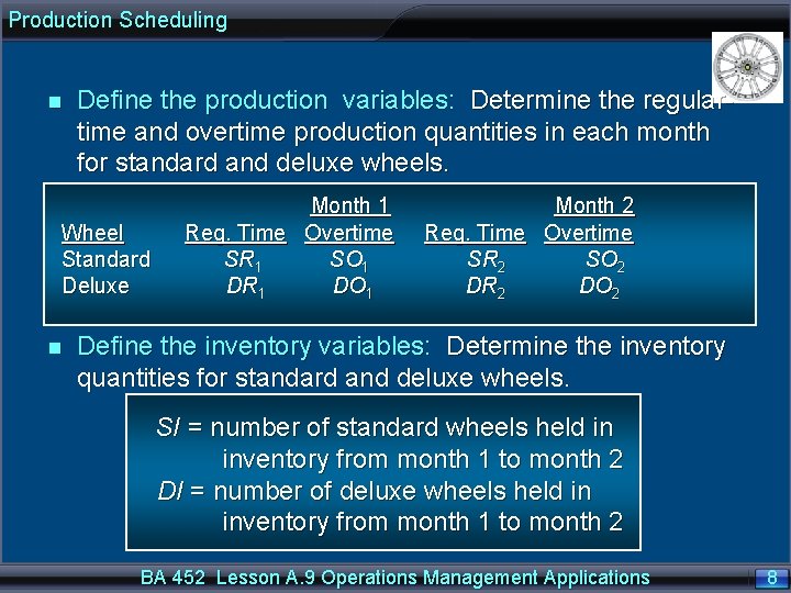
Production Scheduling n Define the production variables: Determine the regulartime and overtime production quantities in each month for standard and deluxe wheels. Wheel Standard Deluxe n Month 1 Reg. Time Overtime SR 1 SO 1 DR 1 DO 1 Month 2 Reg. Time Overtime SR 2 SO 2 DR 2 DO 2 Define the inventory variables: Determine the inventory quantities for standard and deluxe wheels. SI = number of standard wheels held in inventory from month 1 to month 2 DI = number of deluxe wheels held in inventory from month 1 to month 2 BA 452 Lesson A. 9 Operations Management Applications 8

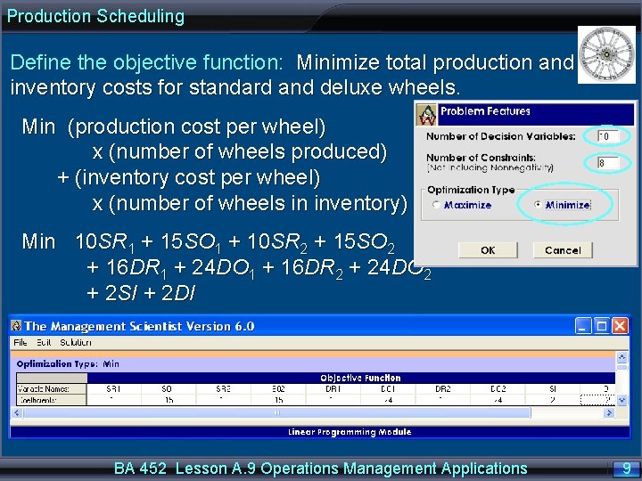
Production Scheduling Define the objective function: Minimize total production and inventory costs for standard and deluxe wheels. Min (production cost per wheel) x (number of wheels produced) + (inventory cost per wheel) x (number of wheels in inventory) Min 10 SR 1 + 15 SO 1 + 10 SR 2 + 15 SO 2 + 16 DR 1 + 24 DO 1 + 16 DR 2 + 24 DO 2 + 2 SI + 2 DI BA 452 Lesson A. 9 Operations Management Applications 9

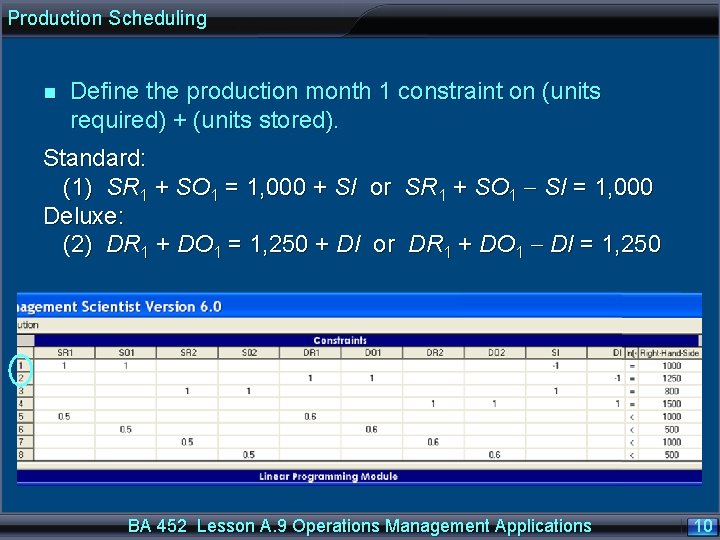
Production Scheduling n Define the production month 1 constraint on (units required) + (units stored). Standard: (1) SR 1 + SO 1 = 1, 000 + SI or SR 1 + SO 1 - SI = 1, 000 Deluxe: (2) DR 1 + DO 1 = 1, 250 + DI or DR 1 + DO 1 - DI = 1, 250 BA 452 Lesson A. 9 Operations Management Applications 10

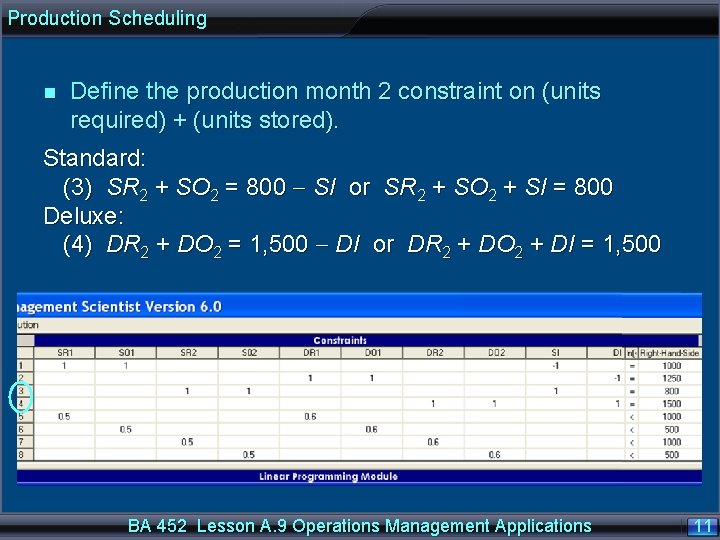
Production Scheduling n Define the production month 2 constraint on (units required) + (units stored). Standard: (3) SR 2 + SO 2 = 800 - SI or SR 2 + SO 2 + SI = 800 Deluxe: (4) DR 2 + DO 2 = 1, 500 - DI or DR 2 + DO 2 + DI = 1, 500 BA 452 Lesson A. 9 Operations Management Applications 11

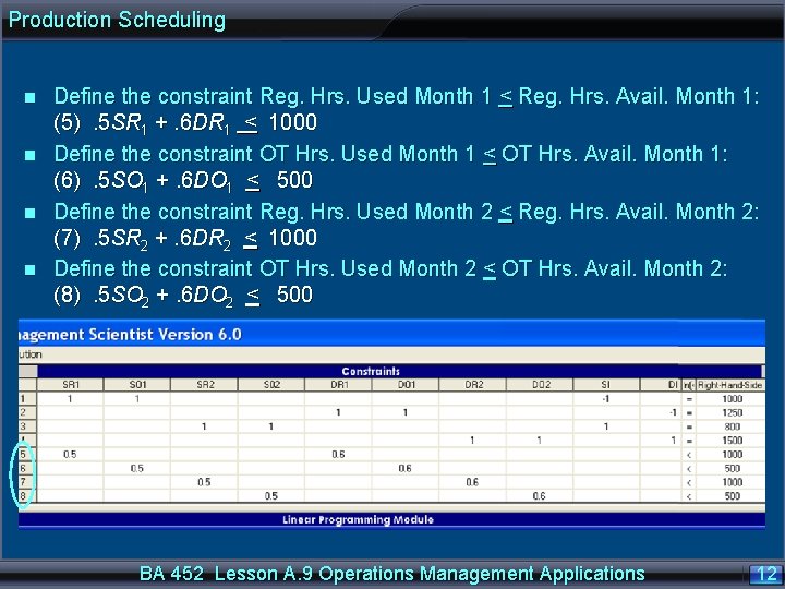
Production Scheduling n n Define the constraint Reg. Hrs. Used Month 1 < Reg. Hrs. Avail. Month 1: (5). 5 SR 1 +. 6 DR 1 < 1000 Define the constraint OT Hrs. Used Month 1 < OT Hrs. Avail. Month 1: (6). 5 SO 1 +. 6 DO 1 < 500 Define the constraint Reg. Hrs. Used Month 2 < Reg. Hrs. Avail. Month 2: (7). 5 SR 2 +. 6 DR 2 < 1000 Define the constraint OT Hrs. Used Month 2 < OT Hrs. Avail. Month 2: (8). 5 SO 2 +. 6 DO 2 < 500 BA 452 Lesson A. 9 Operations Management Applications 12

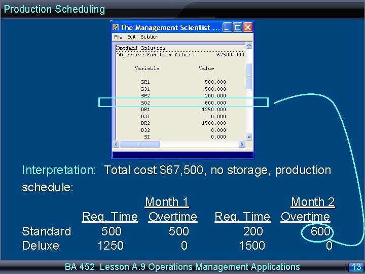
Production Scheduling Interpretation: Total cost $67, 500, no storage, production schedule: Month 1 Month 2 Reg. Time Overtime Standard 500 200 600 Deluxe 1250 0 1500 0 BA 452 Lesson A. 9 Operations Management Applications 13

Production Scheduling with Dynamic Inventory BA 452 Lesson A. 9 Operations Management Applications 14

Production Scheduling with Dynamic Inventory Overview Production Scheduling Problems with Dynamic Inventory help managers find an efficient low-cost production schedule for one or more products over several time periods (weeks or months). A production scheduling problem is resource-allocation problem for each of several periods in the future. Complex problems consider more than two time periods, so there are many periods of inventory. BA 452 Lesson A. 9 Operations Management Applications 15

Production Scheduling with Dynamic Inventory Question: Wilson Sporting Goods produces baseballs. Wilson must decide how many baseballs to produce each month. It has decided to use a 6 -month planning horizon. n The forecasted demands for the next 6 months are 10, 000; 15, 000; 30, 000; 35, 000; 25, 000; and 10, 000. n Wilson wants to meet these demands on time, knowing that it currently has 5, 000 baseballs in inventory and that it can use a given month’s production to help meet the demand for that month. n During each month there is enough production capacity to produce up to 30, 000 baseballs, and there is enough storage capacity to store up to 10, 000 baseballs at the end of the month, after demand has occurred. BA 452 Lesson A. 9 Operations Management Applications 16

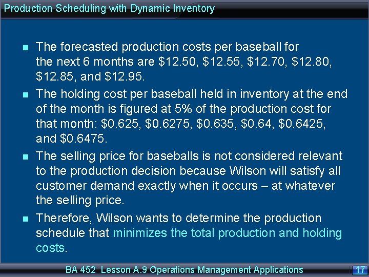
Production Scheduling with Dynamic Inventory n n The forecasted production costs per baseball for the next 6 months are $12. 50, $12. 55, $12. 70, $12. 85, and $12. 95. The holding cost per baseball held in inventory at the end of the month is figured at 5% of the production cost for that month: $0. 625, $0. 6275, $0. 635, $0. 6425, and $0. 6475. The selling price for baseballs is not considered relevant to the production decision because Wilson will satisfy all customer demand exactly when it occurs – at whatever the selling price. Therefore, Wilson wants to determine the production schedule that minimizes the total production and holding costs. BA 452 Lesson A. 9 Operations Management Applications 17

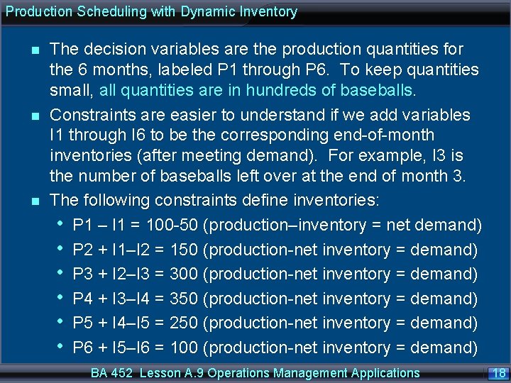
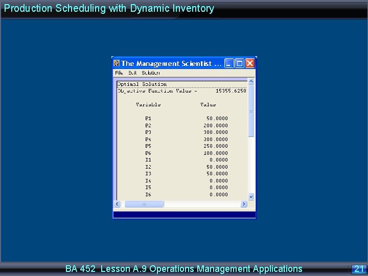
Production Scheduling with Dynamic Inventory n n n The decision variables are the production quantities for the 6 months, labeled P 1 through P 6. To keep quantities small, all quantities are in hundreds of baseballs. Constraints are easier to understand if we add variables I 1 through I 6 to be the corresponding end-of-month inventories (after meeting demand). For example, I 3 is the number of baseballs left over at the end of month 3. The following constraints define inventories: • P 1 – I 1 = 100 -50 (production–inventory = net demand) • P 2 + I 1–I 2 = 150 (production-net inventory = demand) • P 3 + I 2–I 3 = 300 (production-net inventory = demand) • P 4 + I 3–I 4 = 350 (production-net inventory = demand) • P 5 + I 4–I 5 = 250 (production-net inventory = demand) • P 6 + I 5–I 6 = 100 (production-net inventory = demand) BA 452 Lesson A. 9 Operations Management Applications 18

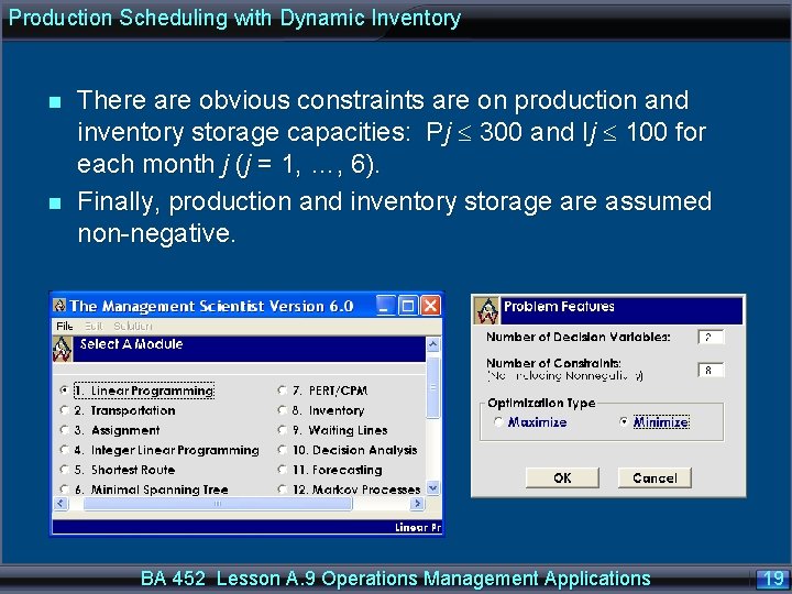
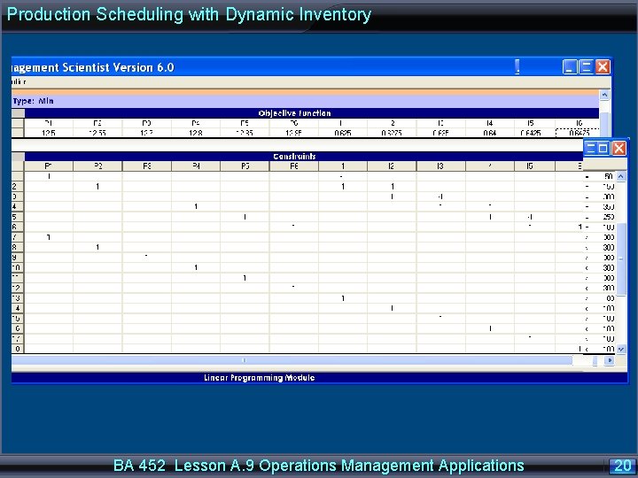
Production Scheduling with Dynamic Inventory n n There are obvious constraints are on production and inventory storage capacities: Pj 300 and Ij 100 for each month j (j = 1, …, 6). Finally, production and inventory storage are assumed non-negative. BA 452 Lesson A. 9 Operations Management Applications 19

Production Scheduling with Dynamic Inventory n There BA 452 Lesson A. 9 Operations Management Applications 20

Production Scheduling with Dynamic Inventory BA 452 Lesson A. 9 Operations Management Applications 21

Workforce Assignment BA 452 Lesson A. 9 Operations Management Applications 22

Workforce Assignment Overview Workforce Assignment Problems are Resource Allocation Problems when labor is one of the resources, and labor allocation has some flexibility; at least some labor can be assigned to more than one department or work center. Workforce Assignment Problems thus help when employees have been cross-trained on two or more jobs or, for instance, when sales personnel can be transferred between stores. BA 452 Lesson A. 9 Operations Management Applications 23

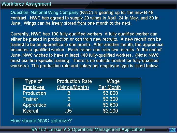
Workforce Assignment Question: National Wing Company (NWC) is gearing up for the new B-48 contract. NWC has agreed to supply 20 wings in April, 24 in May, and 30 in June. Wings can be freely stored from one month to the next. Currently, NWC has 100 fully-qualified workers. A fully qualified worker can either be placed in production or can train new recruits. A new recruit can be trained to be an apprentice in one month. After another month, the apprentice becomes a qualified worker. Each trainer can train two recruits. At the end of June, NWC wishes to have at least 140 fully-qualified workers. (Note: NWC must use firm-specific training. There is no outside market for fully-qualified workers. ) The production rate and salary per employee type is listed below. Type of Employee Production Trainer Apprentice Recruit Production Rate (Wings/Month). 6. 3. 4. 05 Wage Per Month $3, 000 $3, 300 $2, 600 $2, 200 How should NWC optimize? BA 452 Lesson A. 9 Operations Management Applications 24

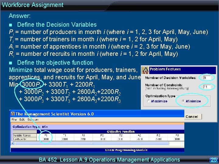
Workforce Assignment Answer: n Define the Decision Variables Pi = number of producers in month i (where i = 1, 2, 3 for April, May, June) Ti = number of trainers in month i (where i = 1, 2 for April, May) Ai = number of apprentices in month i (where i = 2, 3 for May, June) Ri = number of recruits in month i (where i = 1, 2 for April, May) n Define the objective function Minimize total wage cost for producers, trainers, apprentices, and recruits for April, May, and June: Min 3000 P 1 + 3300 T 1 + 2200 R 1 + 3000 P 2 + 3300 T 2 + 2600 A 2+2200 R 2 + 3000 P 3 + 3300 T 3 + 2600 A 3+2200 R 3 BA 452 Lesson A. 9 Operations Management Applications 25

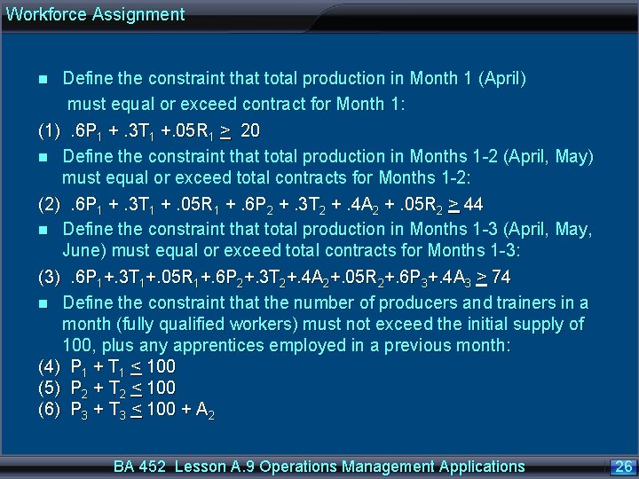
Workforce Assignment Define the constraint that total production in Month 1 (April) must equal or exceed contract for Month 1: (1). 6 P 1 +. 3 T 1 +. 05 R 1 > 20 n Define the constraint that total production in Months 1 -2 (April, May) must equal or exceed total contracts for Months 1 -2: (2). 6 P 1 +. 3 T 1 +. 05 R 1 +. 6 P 2 +. 3 T 2 +. 4 A 2 +. 05 R 2 > 44 n Define the constraint that total production in Months 1 -3 (April, May, June) must equal or exceed total contracts for Months 1 -3: (3). 6 P 1+. 3 T 1+. 05 R 1+. 6 P 2+. 3 T 2+. 4 A 2+. 05 R 2+. 6 P 3+. 4 A 3 > 74 n Define the constraint that the number of producers and trainers in a month (fully qualified workers) must not exceed the initial supply of 100, plus any apprentices employed in a previous month: (4) P 1 + T 1 < 100 (5) P 2 + T 2 < 100 (6) P 3 + T 3 < 100 + A 2 n BA 452 Lesson A. 9 Operations Management Applications 26

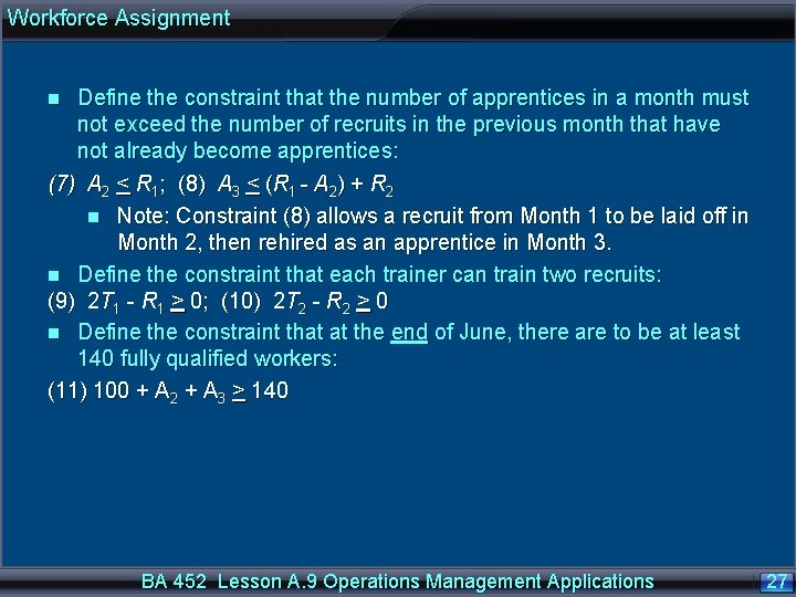
Workforce Assignment Define the constraint that the number of apprentices in a month must not exceed the number of recruits in the previous month that have not already become apprentices: (7) A 2 < R 1; (8) A 3 < (R 1 - A 2) + R 2 n Note: Constraint (8) allows a recruit from Month 1 to be laid off in Month 2, then rehired as an apprentice in Month 3. n Define the constraint that each trainer can train two recruits: (9) 2 T 1 - R 1 > 0; (10) 2 T 2 - R 2 > 0 n Define the constraint that at the end of June, there are to be at least 140 fully qualified workers: (11) 100 + A 2 + A 3 > 140 n BA 452 Lesson A. 9 Operations Management Applications 27

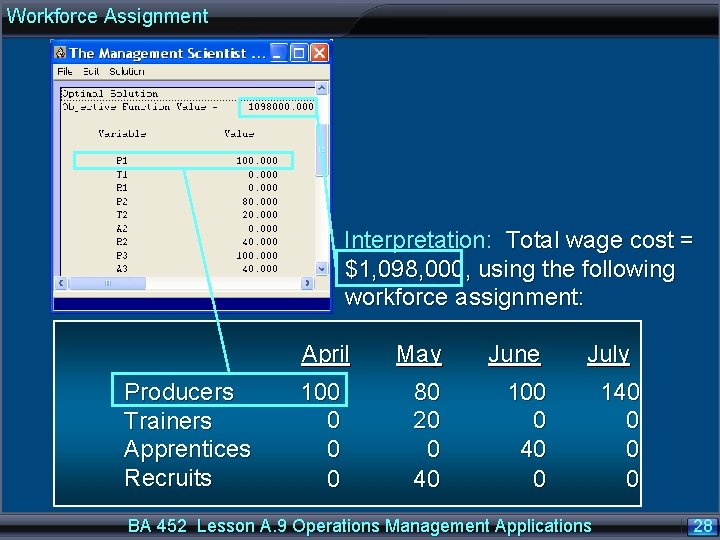
Workforce Assignment Interpretation: Total wage cost = $1, 098, 000, using the following workforce assignment: April Producers Trainers Apprentices Recruits 100 0 May June 80 20 0 40 100 0 40 0 July BA 452 Lesson A. 9 Operations Management Applications 140 0 28

Make or Buy BA 452 Lesson A. 9 Operations Management Applications 29

Make or Buy Overview Make or Buy Problems are Linear Programming Profit Maximization problems when outputs are fixed and when inputs can be either made or bought. Make or Buy Problems thus help production managers to minimize cost by comparing, for some inputs, the lower cost of manufacturing those inputs (rather then buying them) to the opportunity cost of the scarce resources used in manufacture. BA 452 Lesson A. 9 Operations Management Applications 30

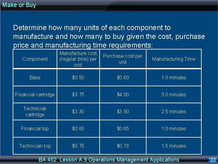
Make or Buy Question: The Janders Company markets business and engineering products. Janders is currently preparing to introduce two new calculators: one for the business market called the Financial Manager, and one for the engineering market called the Technician. Each calculator has three components: a base, an electronic cartridge, and a faceplate or top. The same base is used for both calculators, but the cartridges and tops are different. All components can be manufactured by the company or purchased from outside suppliers. BA 452 Lesson A. 9 Operations Management Applications 31

Make or Buy Company forecasters indicate that 3000 Financial Manager calculators and 2000 Technician calculators will be demanded. However, manufacturing capacity is limited. The company has 200 hours of regular time manufacturing time and 50 hours of overtime that can be scheduled for the calculators. Overtime involves a premium at the additional cost of $9 per hour. BA 452 Lesson A. 9 Operations Management Applications 32

Make or Buy Determine how many units of each component to manufacture and how many to buy given the cost, purchase price and manufacturing time requirements: Component Manufacture cost (regular time) per unit Purchase cost per unit Manufacturing Time Base $0. 50 $0. 60 1. 0 minutes Financial cartridge $3. 75 $4. 00 3. 0 minutes Technician cartridge $3. 30 $3. 90 2. 5 minutes Financial top $0. 60 $0. 65 1. 0 minutes Technician top $0. 75 $0. 78 1. 5 minutes BA 452 Lesson A. 9 Operations Management Applications 33

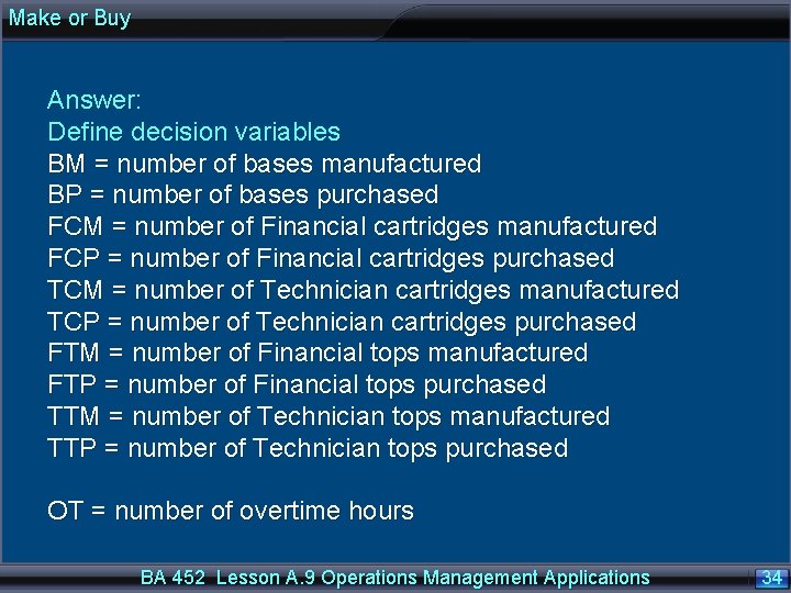
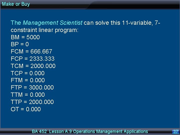
Make or Buy Answer: Define decision variables BM = number of bases manufactured BP = number of bases purchased FCM = number of Financial cartridges manufactured FCP = number of Financial cartridges purchased TCM = number of Technician cartridges manufactured TCP = number of Technician cartridges purchased FTM = number of Financial tops manufactured FTP = number of Financial tops purchased TTM = number of Technician tops manufactured TTP = number of Technician tops purchased OT = number of overtime hours BA 452 Lesson A. 9 Operations Management Applications 34

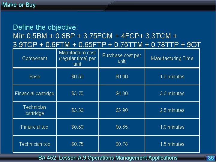
Make or Buy Define the objective: Min 0. 5 BM + 0. 6 BP + 3. 75 FCM + 4 FCP+ 3. 3 TCM + 3. 9 TCP + 0. 6 FTM + 0. 65 FTP + 0. 75 TTM + 0. 78 TTP + 9 OT Component Manufacture cost (regular time) per unit Purchase cost per unit Manufacturing Time Base $0. 50 $0. 60 1. 0 minutes Financial cartridge $3. 75 $4. 00 3. 0 minutes Technician cartridge $3. 30 $3. 90 2. 5 minutes Financial top $0. 60 $0. 65 1. 0 minutes Technician top $0. 75 $0. 78 1. 5 minutes BA 452 Lesson A. 9 Operations Management Applications 35

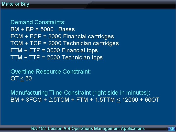
Make or Buy Demand Constraints: BM + BP = 5000 Bases FCM + FCP = 3000 Financial cartridges TCM + TCP = 2000 Technician cartridges FTM + FTP = 3000 Financial tops TTM + TTP = 2000 Technician tops Overtime Resource Constraint: OT < 50 Manufacturing Time Constraint (right-side in minutes): BM + 3 FCM + 2. 5 TCM + FTM + 1. 5 TTM < 12000 + 60 OT BA 452 Lesson A. 9 Operations Management Applications 36

Make or Buy The Management Scientist can solve this 11 -variable, 7 constraint linear program: BM = 5000 BP = 0 FCM = 666. 667 FCP = 2333. 333 TCM = 2000. 000 TCP = 0. 000 FTM = 0. 000 FTP = 3000. 000 TTM = 0. 000 TTP = 2000. 000 OT = 0. 000 BA 452 Lesson A. 9 Operations Management Applications 37

Product Mix BA 452 Lesson A. 9 Operations Management Applications 38

Product Mix Overview Product Mix Problems are Resource Allocation Problems when outputs have different physical characteristics. Product Mix Problems thus help managers determine the production levels that meet demand requirements, given limitations on production capacity and labor capacity, to maximize profit or minimize cost. BA 452 Lesson A. 9 Operations Management Applications 39

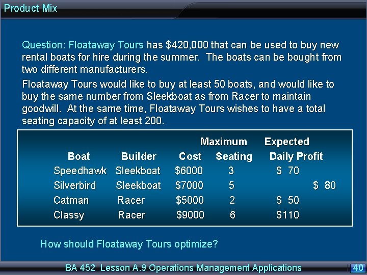
Product Mix Question: Floataway Tours has $420, 000 that can be used to buy new rental boats for hire during the summer. The boats can be bought from two different manufacturers. Floataway Tours would like to buy at least 50 boats, and would like to buy the same number from Sleekboat as from Racer to maintain goodwill. At the same time, Floataway Tours wishes to have a total seating capacity of at least 200. Boat Builder Speedhawk Sleekboat Silverbird Sleekboat Catman Racer Classy Racer Maximum Cost Seating $6000 3 $7000 5 $5000 2 $9000 6 Expected Daily Profit $ 70 $ 80 $ 50 $110 How should Floataway Tours optimize? BA 452 Lesson A. 9 Operations Management Applications 40

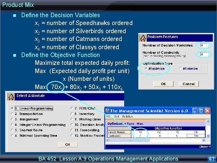
Product Mix n n Define the Decision Variables x 1 = number of Speedhawks ordered x 2 = number of Silverbirds ordered x 3 = number of Catmans ordered x 4 = number of Classys ordered Define the Objective Function Maximize total expected daily profit: Max (Expected daily profit per unit) x (Number of units) Max 70 x 1 + 80 x 2 + 50 x 3 + 110 x 4 BA 452 Lesson A. 9 Operations Management Applications 41

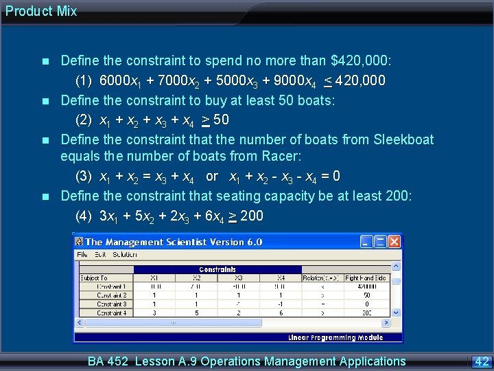
Product Mix n n Define the constraint to spend no more than $420, 000: (1) 6000 x 1 + 7000 x 2 + 5000 x 3 + 9000 x 4 < 420, 000 Define the constraint to buy at least 50 boats: (2) x 1 + x 2 + x 3 + x 4 > 50 Define the constraint that the number of boats from Sleekboat equals the number of boats from Racer: (3) x 1 + x 2 = x 3 + x 4 or x 1 + x 2 - x 3 - x 4 = 0 Define the constraint that seating capacity be at least 200: (4) 3 x 1 + 5 x 2 + 2 x 3 + 6 x 4 > 200 BA 452 Lesson A. 9 Operations Management Applications 42

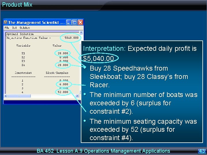
Product Mix Interpretation: Expected daily profit is $5, 040. 00. • Buy 28 Speedhawks from Sleekboat; buy 28 Classy’s from Racer. • The minimum number of boats was exceeded by 6 (surplus for constraint #2). • The minimum seating capacity was exceeded by 52 (surplus for constraint #4). BA 452 Lesson A. 9 Operations Management Applications 43

Blending with Weight Constraints BA 452 Lesson A. 9 Operations Management Applications 44

Blending with Weight Constraints Overview Blending Problems with Weight Constraints help production managers blend resources to produce goods of a specific weight at minimum cost. BA 452 Lesson A. 9 Operations Management Applications 45

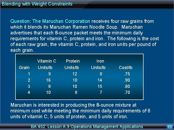
Blending with Weight Constraints Question: The Maruchan Corporation receives four raw grains from which it blends its Maruchan Ramen Noodle Soup. Maruchan advertises that each 8 -ounce packet meets the minimum daily requirements for vitamin C, protein and iron. The following is the cost of each raw grain, the vitamin C, protein, and iron units per pound of each grain. Grain 1 2 3 4 Vitamin C Units/lb 9 16 8 10 Protein Units/lb 12 10 10 8 Iron Units/lb 0 14 15 7 Cost/lb. 75. 90. 80. 70 Maruchan is interested in producing the 8 -ounce mixture at minimum cost while meeting the minimum daily requirements of 6 units of vitamin C, 5 units of protein, and 5 units of iron. BA 452 Lesson A. 9 Operations Management Applications 46

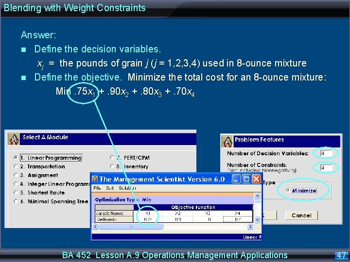
Blending with Weight Constraints Answer: n Define the decision variables. xj = the pounds of grain j (j = 1, 2, 3, 4) used in 8 -ounce mixture n Define the objective. Minimize the total cost for an 8 -ounce mixture: Min. 75 x 1 +. 90 x 2 +. 80 x 3 +. 70 x 4 BA 452 Lesson A. 9 Operations Management Applications 47

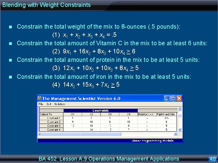
Blending with Weight Constraints n n Constrain the total weight of the mix to 8 -ounces (. 5 pounds): (1) x 1 + x 2 + x 3 + x 4 =. 5 Constrain the total amount of Vitamin C in the mix to be at least 6 units: (2) 9 x 1 + 16 x 2 + 8 x 3 + 10 x 4 > 6 Constrain the total amount of protein in the mix to be at least 5 units: (3) 12 x 1 + 10 x 2 + 10 x 3 + 8 x 4 > 5 Constrain the total amount of iron in the mix to be at least 5 units: (4) 14 x 2 + 15 x 3 + 7 x 4 > 5 BA 452 Lesson A. 9 Operations Management Applications 48

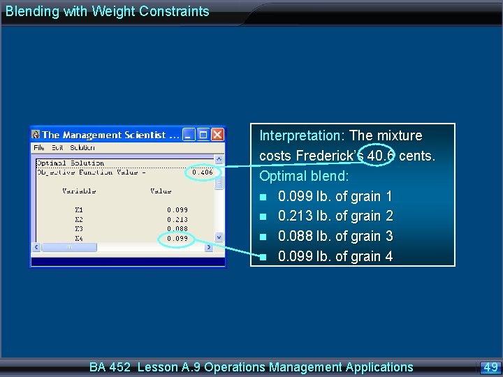
Blending with Weight Constraints Interpretation: The mixture costs Frederick’s 40. 6 cents. Optimal blend: n 0. 099 lb. of grain 1 n 0. 213 lb. of grain 2 n 0. 088 lb. of grain 3 n 0. 099 lb. of grain 4 BA 452 Lesson A. 9 Operations Management Applications 49

BA 452 Analysis Quantitative End of Lesson A. 9 BA 452 Lesson A. 9 Operations Management Applications 50