RDF3 X a RISC style Engine for RDF

RDF-3 X: a RISC style Engine for RDF Ref: Thomas Neumann and Gerhard Weikum [PVLDB’ 08 ] Presented by: Pankaj Vanwari Course: Advanced Databases (CS 632)

Motivation • RDF(Resource Description Framework ) is schema-free structured information. • Increasingly popular in context of – Knowledge bases – Semantic Web – Life-Sciences and Online communities. • Managing large-scale RDF data includes challenges for – Storage layout, indexing and querying

Overview • • • Introduction to RDF and SPARQL Storage of RDF data Query Translation and Processing Query Optimization Evaluation Conclusion

Introduction to RDF • Standard model for data interchange on the Web. • Allows structured and semi-structured data to be mixed, exposed, and shared. • Conceptually a labeled graph – Linking structure forms a directed labeled graph where the edges represent the named link between two resources that are represented by the graph nodes. • Graph is stored as collection of facts. Each edge represents a fact (triple in RDF notation) – Triples have the form (subject; predicate; object)

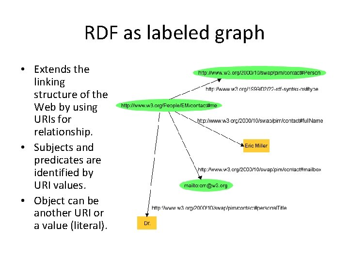
RDF as labeled graph • Extends the linking structure of the Web by using URIs for relationship. • Subjects and predicates are identified by URI values. • Object can be another URI or a value (literal).

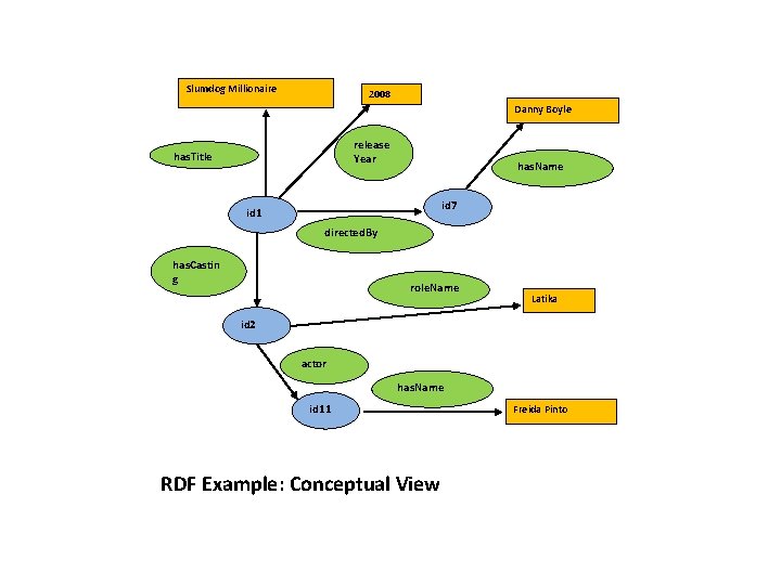
Slumdog Millionaire 2008 Danny Boyle release Year has. Title has. Name id 7 id 1 directed. By has. Castin g role. Name Latika id 2 actor has. Name id 11 RDF Example: Conceptual View Freida Pinto

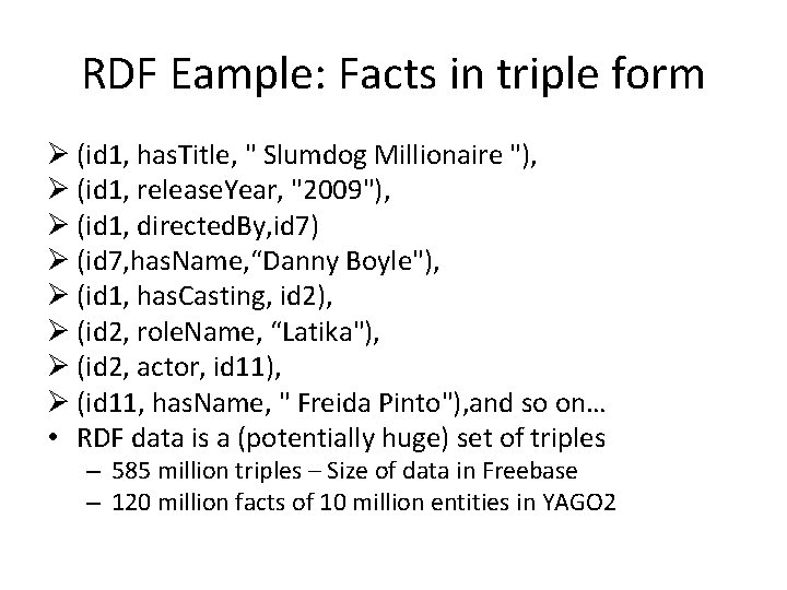
RDF Eample: Facts in triple form Ø (id 1, has. Title, " Slumdog Millionaire "), Ø (id 1, release. Year, "2009"), Ø (id 1, directed. By, id 7) Ø (id 7, has. Name, “Danny Boyle"), Ø (id 1, has. Casting, id 2), Ø (id 2, role. Name, “Latika"), Ø (id 2, actor, id 11), Ø (id 11, has. Name, " Freida Pinto"), and so on… • RDF data is a (potentially huge) set of triples – 585 million triples – Size of data in Freebase – 120 million facts of 10 million entities in YAGO 2

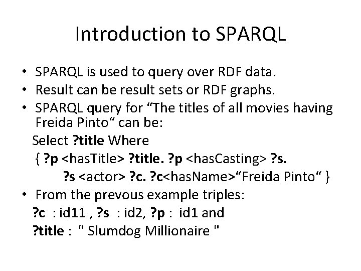
Introduction to SPARQL • SPARQL is used to query over RDF data. • Result can be result sets or RDF graphs. • SPARQL query for “The titles of all movies having Freida Pinto“ can be: Select ? title Where { ? p <has. Title> ? title. ? p <has. Casting> ? s <actor> ? c<has. Name>“Freida Pinto“ } • From the prevous example triples: ? c : id 11 , ? s : id 2, ? p : id 1 and ? title : " Slumdog Millionaire "

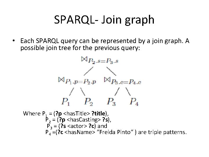
SPARQL- Join graph • Each SPARQL query can be represented by a join graph. A possible join tree for the previous query: Where P 1 = (? p <has. Title> ? title), P 2 = (? p <has. Casting> ? s), P 3 = (? s <actor> ? c) and P 4 =(? c <has. Name> “Freida Pinto“ ) are triple patterns.

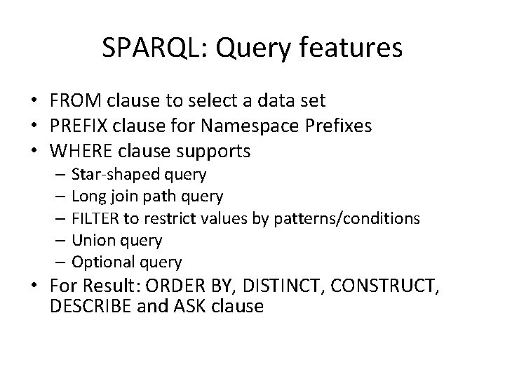
SPARQL: Query features • FROM clause to select a data set • PREFIX clause for Namespace Prefixes • WHERE clause supports – Star-shaped query – Long join path query – FILTER to restrict values by patterns/conditions – Union query – Optional query • For Result: ORDER BY, DISTINCT, CONSTRUCT, DESCRIBE and ASK clause

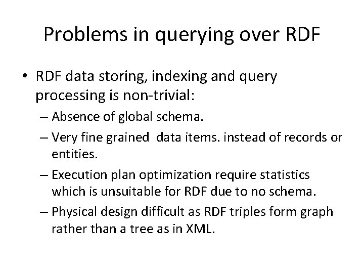
Problems in querying over RDF • RDF data storing, indexing and query processing is non-trivial: – Absence of global schema. – Very fine grained data items. instead of records or entities. – Execution plan optimization require statistics which is unsuitable for RDF due to no schema. – Physical design difficult as RDF triples form graph rather than a tree as in XML.

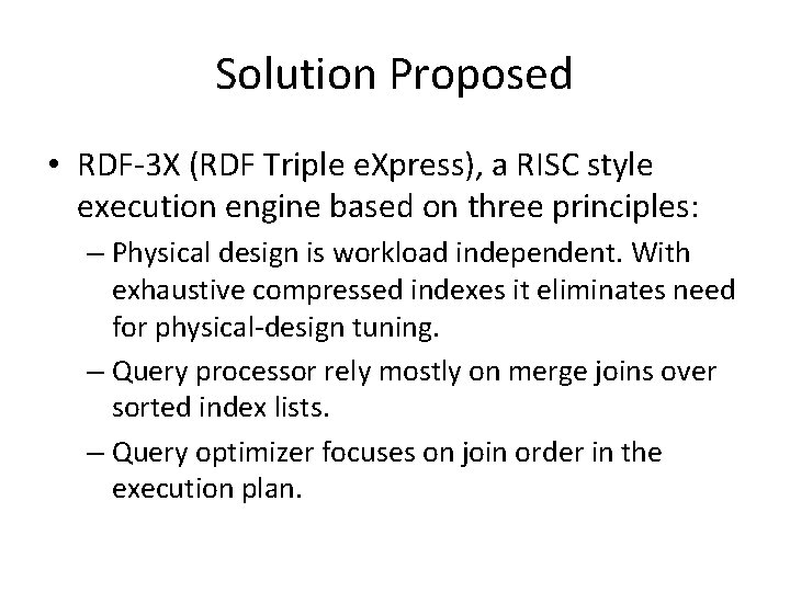
Solution Proposed • RDF-3 X (RDF Triple e. Xpress), a RISC style execution engine based on three principles: – Physical design is workload independent. With exhaustive compressed indexes it eliminates need for physical-design tuning. – Query processor rely mostly on merge joins over sorted index lists. – Query optimizer focuses on join order in the execution plan.

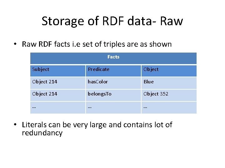
Storage of RDF data- Raw • Raw RDF facts i. e set of triples are as shown Facts Subject Predicate Object 214 has. Color Blue Object 214 belongs. To Object 352 … … … • Literals can be very large and contains lot of redundancy

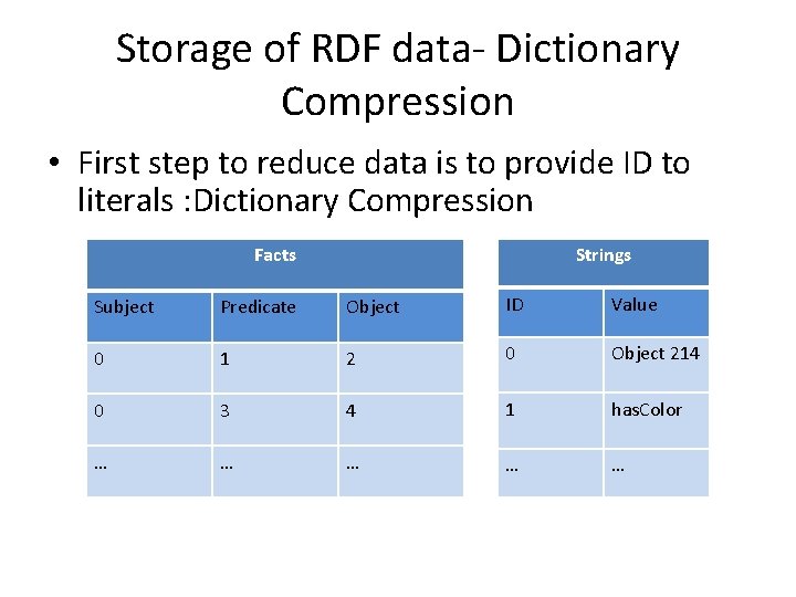
Storage of RDF data- Dictionary Compression • First step to reduce data is to provide ID to literals : Dictionary Compression Facts Strings Subject Predicate Object ID Value 0 1 2 0 Object 214 0 3 4 1 has. Color … … …

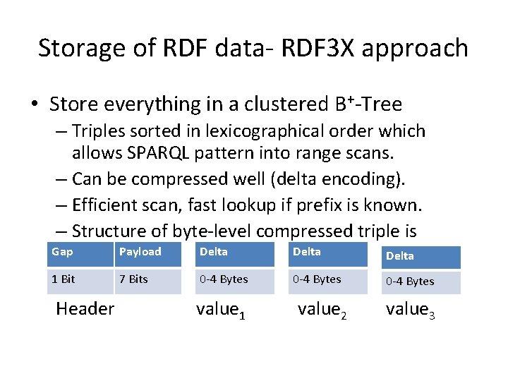
Storage of RDF data- RDF 3 X approach • Store everything in a clustered B+-Tree – Triples sorted in lexicographical order which allows SPARQL pattern into range scans. – Can be compressed well (delta encoding). – Efficient scan, fast lookup if prefix is known. – Structure of byte-level compressed triple is Gap Payload Delta 1 Bit 7 Bits 0 -4 Bytes Header value 1 value 2 value 3

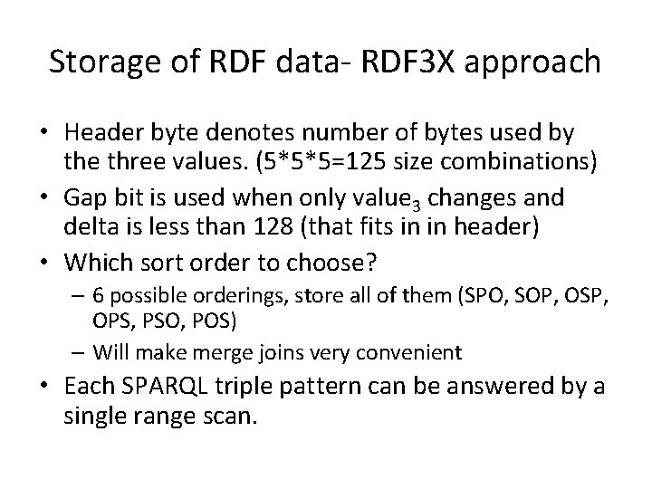
Storage of RDF data- RDF 3 X approach • Header byte denotes number of bytes used by the three values. (5*5*5=125 size combinations) • Gap bit is used when only value 3 changes and delta is less than 128 (that fits in in header) • Which sort order to choose? – 6 possible orderings, store all of them (SPO, SOP, OSP, OPS, PSO, POS) – Will make merge joins very convenient • Each SPARQL triple pattern can be answered by a single range scan.

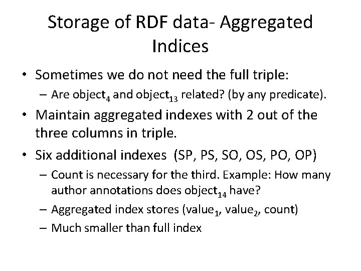
Storage of RDF data- Aggregated Indices • Sometimes we do not need the full triple: – Are object 4 and object 13 related? (by any predicate). • Maintain aggregated indexes with 2 out of the three columns in triple. • Six additional indexes (SP, PS, SO, OS, PO, OP) – Count is necessary for the third. Example: How many author annotations does object 14 have? – Aggregated index stores (value 1, value 2, count) – Much smaller than full index

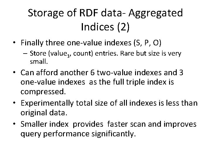
Storage of RDF data- Aggregated Indices (2) • Finally three one-value indexes (S, P, O) – Store (value 1, count) entries. Rare but size is very small. • Can afford another 6 two-value indexes and 3 one-value indexes as the full triple index is compressed. • Experimentally total size of all indexes is less than original data. • Smaller index provides faster scan and improves query performance significantly.

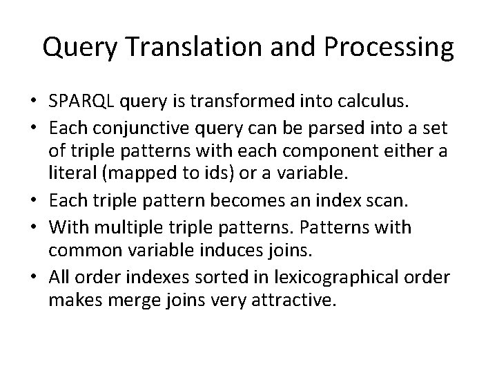
Query Translation and Processing • SPARQL query is transformed into calculus. • Each conjunctive query can be parsed into a set of triple patterns with each component either a literal (mapped to ids) or a variable. • Each triple pattern becomes an index scan. • With multiple triple patterns. Patterns with common variable induces joins. • All order indexes sorted in lexicographical order makes merge joins very attractive.

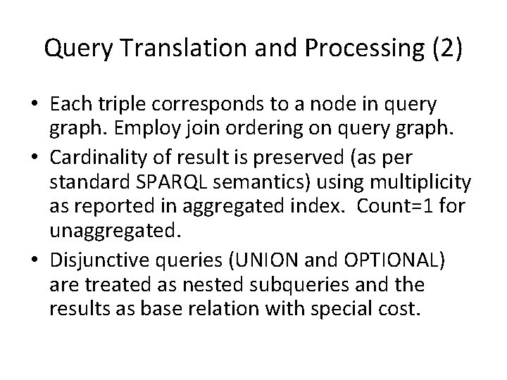
Query Translation and Processing (2) • Each triple corresponds to a node in query graph. Employ join ordering on query graph. • Cardinality of result is preserved (as per standard SPARQL semantics) using multiplicity as reported in aggregated index. Count=1 for unaggregated. • Disjunctive queries (UNION and OPTIONAL) are treated as nested subqueries and the results as base relation with special cost.

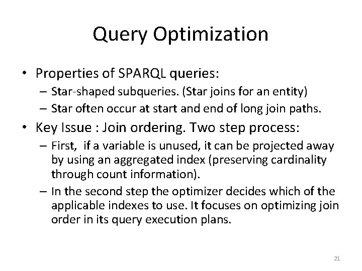
Query Optimization • Properties of SPARQL queries: – Star-shaped subqueries. (Star joins for an entity) – Star often occur at start and end of long join paths. • Key Issue : Join ordering. Two step process: – First, if a variable is unused, it can be projected away by using an aggregated index (preserving cardinality through count information). – In the second step the optimizer decides which of the applicable indexes to use. It focuses on optimizing join order in its query execution plans. 21

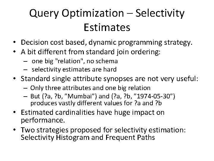
Query Optimization – Selectivity Estimates • Decision cost based, dynamic programming strategy. • A bit different from standard join ordering: – one big "relation", no schema – selectivity estimates are hard • Standard single attribute synopses are not very useful: – Only three attributes and one big relation – But (? a, ? b, ”Mumbai”) and (? a, ? b, ” 1974 -05 -30”) produces vastly different values for ? a and ? b • Estimated cardinalities have huge impact on performance. • Two strategies proposed for selectivity estimation: Selectivity Histogram and Frequent Paths

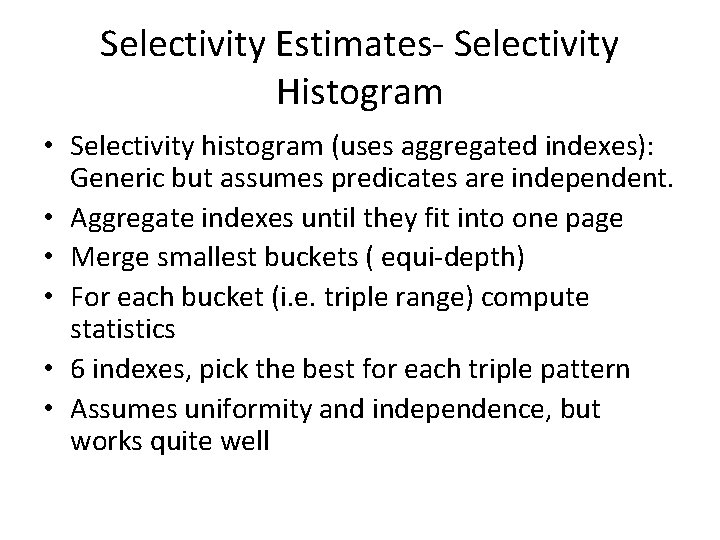
Selectivity Estimates- Selectivity Histogram • Selectivity histogram (uses aggregated indexes): Generic but assumes predicates are independent. • Aggregate indexes until they fit into one page • Merge smallest buckets ( equi-depth) • For each bucket (i. e. triple range) compute statistics • 6 indexes, pick the best for each triple pattern • Assumes uniformity and independence, but works quite well

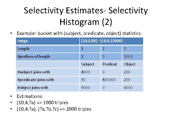
Selectivity Estimates- Selectivity Histogram (2) • Example: bucket with (subject, predicate, object) statistics range (10, 2, 30) - (10, 5, 12000) Length 1 2 3 #prefixes of length 1 3 3000 Subject Predicat Object #subject joins with 4000 0 200 #predicate joins with 50 400000 200 #object joins with 6000 0 9000 • Estimations: • (10, 4, ? a) => 1000 triples • (10, 4, ? a), (? a, ? b, ? c) => 2000 triples

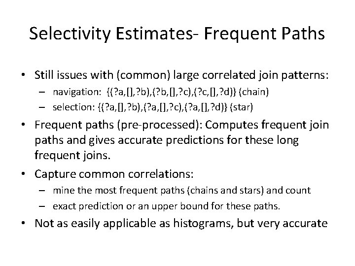
Selectivity Estimates- Frequent Paths • Still issues with (common) large correlated join patterns: – navigation: {(? a, [], ? b), (? b, [], ? c), (? c, [], ? d)} (chain) – selection: {(? a, [], ? b), (? a, [], ? c), (? a, [], ? d)} (star) • Frequent paths (pre-processed): Computes frequent join paths and gives accurate predictions for these long frequent joins. • Capture common correlations: – mine the most frequent paths (chains and stars) and count – exact prediction or an upper bound for these paths. • Not as easily applicable as histograms, but very accurate

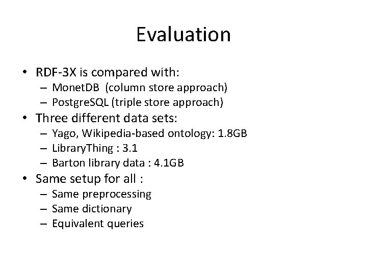
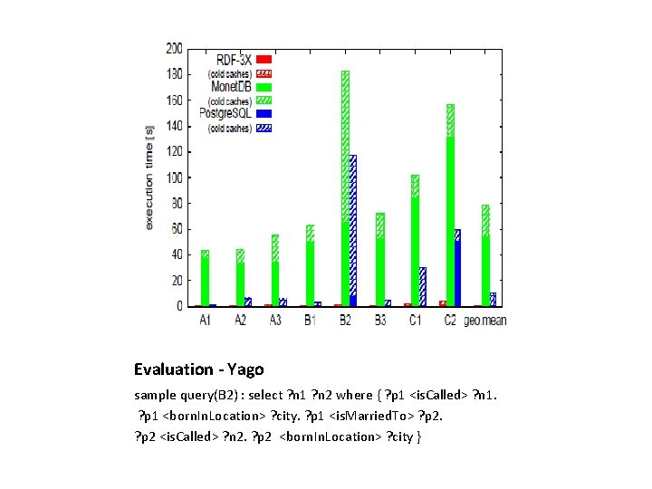
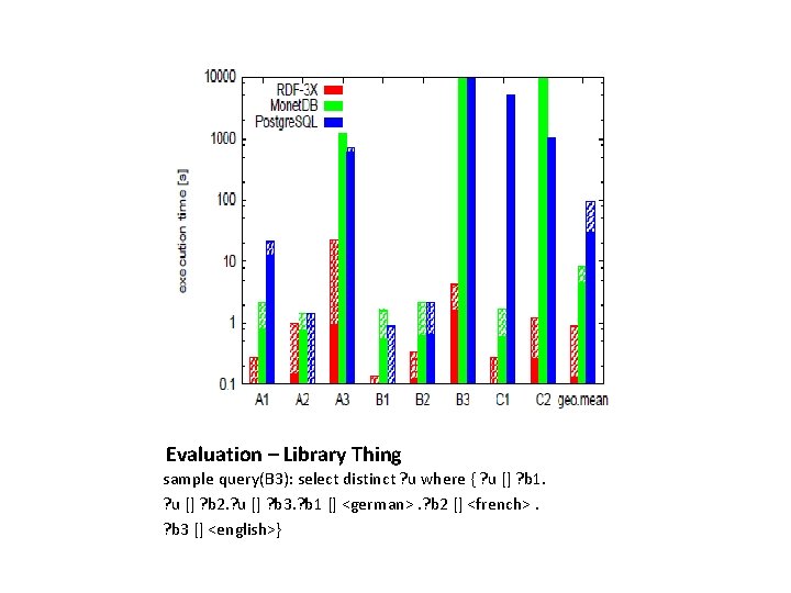
Evaluation • RDF-3 X is compared with: – Monet. DB (column store approach) – Postgre. SQL (triple store approach) • Three different data sets: – Yago, Wikipedia-based ontology: 1. 8 GB – Library. Thing : 3. 1 – Barton library data : 4. 1 GB • Same setup for all : – Same preprocessing – Same dictionary – Equivalent queries

Evaluation - Yago sample query(B 2) : select ? n 1 ? n 2 where { ? p 1 <is. Called> ? n 1. ? p 1 <born. In. Location> ? city. ? p 1 <is. Married. To> ? p 2 <is. Called> ? n 2. ? p 2 <born. In. Location> ? city }

Evaluation – Library Thing sample query(B 3): select distinct ? u where { ? u [] ? b 1. ? u [] ? b 2. ? u [] ? b 3. ? b 1 [] <german>. ? b 2 [] <french>. ? b 3 [] <english>}

Evaluation – Barton Data Set [VLDB 07] sample query (Q 5) select ? a ? c where { ? a <origin> <marcorg/DLC>. ? a <records> ? b <type >? c. filter (? c != <Text>) }

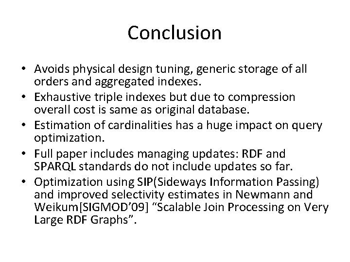
Conclusion • Avoids physical design tuning, generic storage of all orders and aggregated indexes. • Exhaustive triple indexes but due to compression overall cost is same as original database. • Estimation of cardinalities has a huge impact on query optimization. • Full paper includes managing updates: RDF and SPARQL standards do not include updates so far. • Optimization using SIP(Sideways Information Passing) and improved selectivity estimates in Newmann and Weikum[SIGMOD’ 09] “Scalable Join Processing on Very Large RDF Graphs”.

Thank You