RDF graph summaries 2014113 1 Graph Summary A

RDF graph summaries 金成 2014/11/3 1

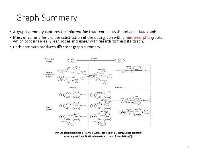
Graph Summary • A graph summary captures the information that represents the original data graph. • Most of summaries are the substitution of the data graph with a homomorphic graph, which contains ideally less nodes and edges with regards to the data graph. • Each approach produces different graph summary. [Picture from Campinas S, Perry T E, Ceccarelli D, et al. Introducing rdf graph summary with application to assisted sparql formulation[C]] 2

Pattern extraction 3

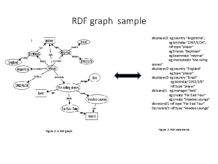
RDF graph sample db: player/1 eg: country “Argentina”; eg: birthday “ 1987/6/24”; rdf: type “player” eg: friends “Beckham” eg: teammate “neymar” eg: instrested. In “the roling stones” db: player/2 eg: country “England” eg: type “player” db: player/3 eg: country ”Brazil” eg: birthday” 1992/2/5” rdf: type “player” db: band/1 eg: manager: ”bob” eg: create “Far East Tour” eg: create “Voodoo Lounge” db: record/1 rdf type “Far East Tour” Db: record/2 rdf: type “Voodoo Lounge” Figure 2: A RDF graph Figure 3: RDF statements

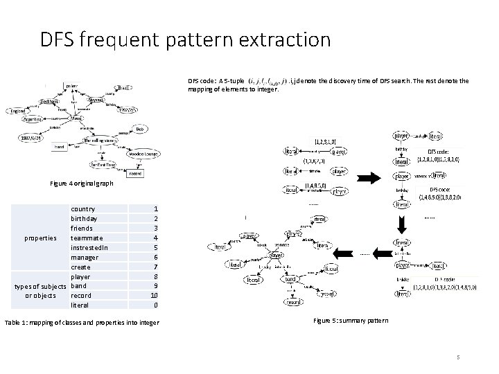
DFS frequent pattern extraction DFS code: A 5 -tuple mapping of elements to integer. . i, j denote the discovery time of DFS search. The rest denote the Figure 4 original graph country birthday friends teammate properties instrested. In manager create player types of subjects band or objects record literal 1 2 3 4 5 6 7 8 9 10 0 Table 1: mapping of classes and properties into integer Figure 5: summary pattern 5

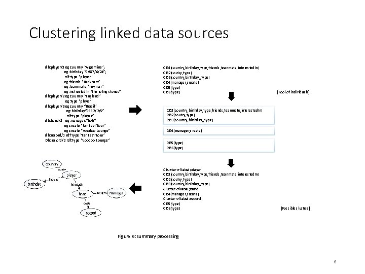
Clustering linked data sources db: player/1 eg: country “Argentina”; eg: birthday “ 1987/6/24”; rdf: type “player” eg: friends “Beckham” eg: teammate “neymar” eg: instrested. In “the roling stones” db: player/2 eg: country “England” eg: type “player” db: player/3 eg: country ”Brazil” eg: birthday” 1992/2/5” rdf: type “player” db: band/1 eg: manager: ”bob” eg: create “Far East Tour” eg: create “Voodoo Lounge” db: record/1 rdf type “Far East Tour” Db: record/2 rdf: type “Voodoo Lounge” CD 1{country, birthday, type, friends, teanmate, interested. In} CD 2{coutry, type} CD 3{country, birthday, , type} CD 4{manager, create} CD 5{type} CD 6{type} [Pool of individuals] CD 1{country, birthday, type, friends, teanmate, interested. In} CD 2{coutry, type} CD 3{country, birthday, , type} CD 4{manager, create} CD 5{type} CD 6{type} C luster of label: player CD 1{country, birthday, type, friends, teanmate, interested. In} CD 2{coutry, type} CD 3{country, birthday, , type} Cluster of label; band CD 4{manager, create} Cluster of label: record CD 5{type} CD 6{type} [Possible clusters] Figure 6: summary processing 6

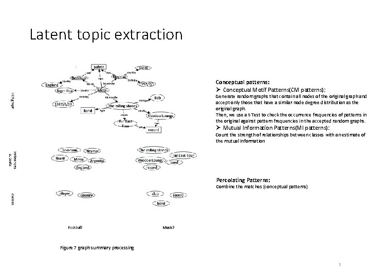
Latent topic extraction Conceptual patterns: Ø Conceptual Motif Patterns(CM patterns): Generate random graphs that contain all nodes of the original graph and accept only those that have a similar node degree distribution as the original graph. Then, we use a t-Test to check the occurrence frequencies of patterns in the original against pattern frequencies in the accepted random graphs. Ø Mutual Information Patterns(MI patterns): Count the strength of relationships between classes with an estimate of the mutual information Percolating Patterns: Combine the matches (conceptual patterns) Figure 7 graph summary processing 7

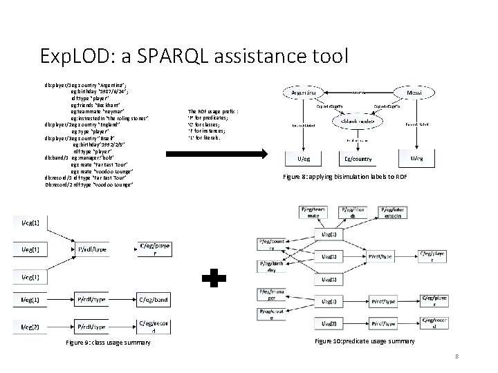
Exp. LOD: a SPARQL assistance tool db: player/1 eg: country “Argentina”; eg: birthday “ 1987/6/24”; rdf: type “player” eg: friends “Beckham” eg: teammate “neymar” eg: instrested. In “the roling stones” db: player/2 eg: country “England” eg: type “player” db: player/3 eg: country ”Brazil” eg: birthday” 1992/2/5” rdf: type “player” db: band/1 eg: manager: ”bob” eg: create “Far East Tour” eg: create “Voodoo Lounge” db: record/1 rdf type “Far East Tour” Db: record/2 rdf: type “Voodoo Lounge” Figure 9: class usage summary The RDF usage prefix : ’P’ for predicates; ’C’ for classes; ’I’ for instances; ’L’ for literals. Figure 8: applying bisimulation labels to RDF Figure 10: predicate usage summary 8

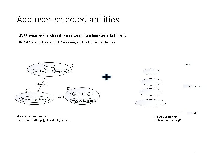
Add user-selected abilities SNAP: grouping nodes based on user-selected attributes and relationships. K-SNAP: on the basis of SNAP, user may control the size of clusters. Figure 11: SNAP summary user defined: {rdf: type}{interested. In, create} Figure 12: k-SNAP different resolution(k) 9

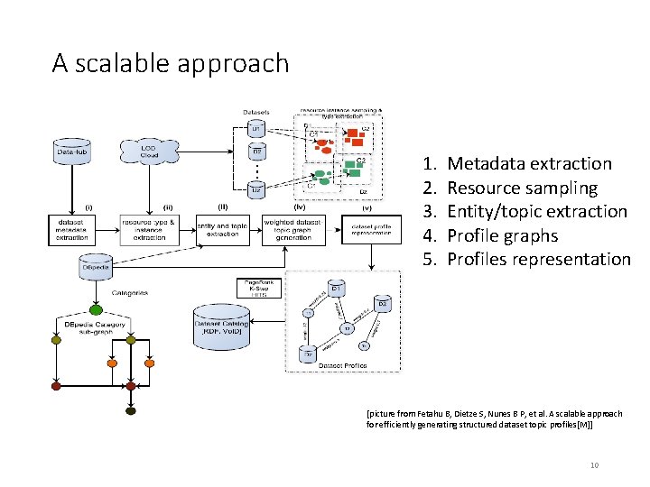
A scalable approach 1. 2. 3. 4. 5. Metadata extraction Resource sampling Entity/topic extraction Profile graphs Profiles representation [picture from Fetahu B, Dietze S, Nunes B P, et al. A scalable approach for efficiently generating structured dataset topic profiles[M]] 10

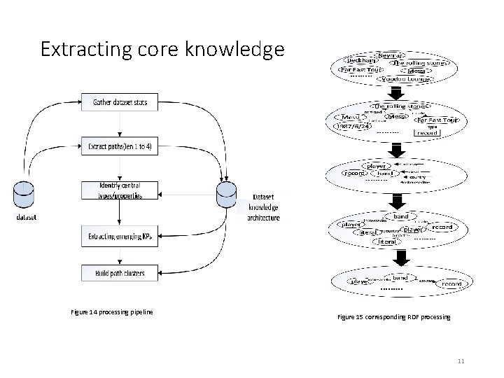
Extracting core knowledge Figure 14 processing pipeline Figure 15 corresponding RDF processing 11

Schema extraction 12

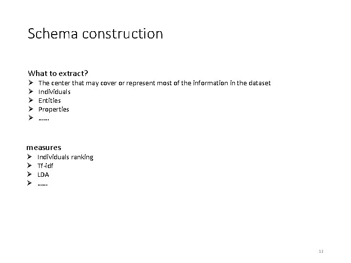
Schema construction What to extract? Ø Ø Ø The center that may cover or represent most of the information in the dataset Individuals Entities Properties …… measures Ø Ø Individuals ranking Tf-idf LDA …… 13

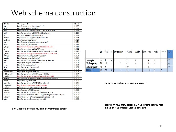
Web schema construction Table 3: web schema content and statics Table 2: list of ontologies found in a e-Commerce dataset [Tables from Ashraf J, Hadzic M. Web schema construction based on web ontology usage analysis[M]] 14

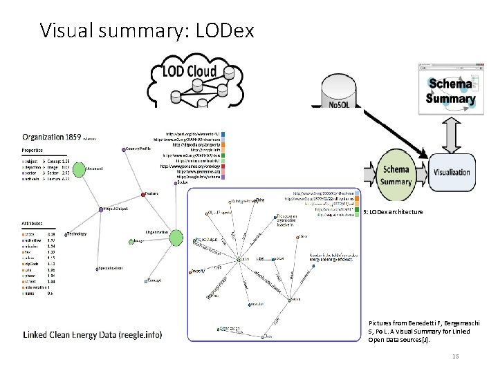
Visual summary: LODex Figure 16: LODex architecture Figure 17: a visual sample Pictures from Benedetti F, Bergamaschi S, Po L. A Visual Summary for Linked Open Data sources[J]. 15

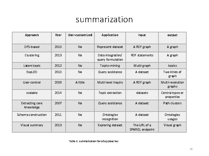
summarization Approach Year User-customized Application input output DFS-based 2010 No Represent dataset A RDF graph A graph Clustering 2013 No Data integration/ query formulation RDF statements A graph Latent topic 2012 No Topics mining Multi-graph topics Exp. LOD 2010 No Query assistance A dataset Two kinds of graph User-control 2008 A little Multi-level inquiry A RDF graph Multi-resolution graphs scalable 2014 No Topic extraction datasets Central types or properties Extracting core knowledge 2007 No Query assistance A dataset Path clusters Schema construction 2011 No Ontologies recognition A dataset Ontologies usages Visual summary 2013 No Exploring dataset The URL of a SPARQL endpoint Visual graph Table 4 summarization for all approaches 16