RD Risks and Overreaction in a Market where

R&D, Risks and Overreaction in a Market where the Book-to-Market Effect is Reputedly Absent Weifeng Hung, Feng Chia Universty, Taiwan Chaoshin Chiao, National Dong Hwa University, Taiwan Tung-Liang Liao, Feng Chia Universty, Taiwan Presenter: Sheng-Tang Huang, Nanya Institute of Technology, Taiwan

Motivation o The absence of the book-to-market effect in the Taiwan stock market has been widely documented in a considerable number of the prior studies. o Is there really the absence of the book-to-market effect in the Taiwan Stock Market?

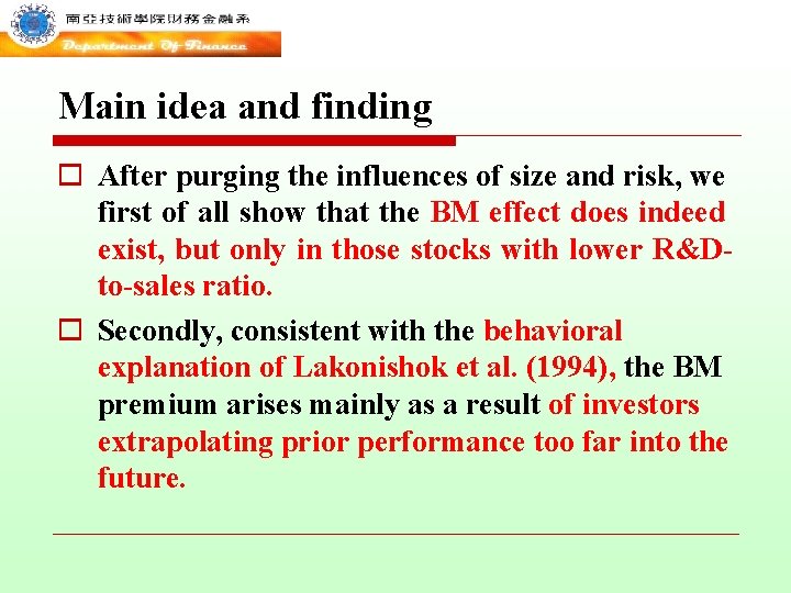
Main idea and finding o After purging the influences of size and risk, we first of all show that the BM effect does indeed exist, but only in those stocks with lower R&Dto-sales ratio. o Secondly, consistent with the behavioral explanation of Lakonishok et al. (1994), the BM premium arises mainly as a result of investors extrapolating prior performance too far into the future.

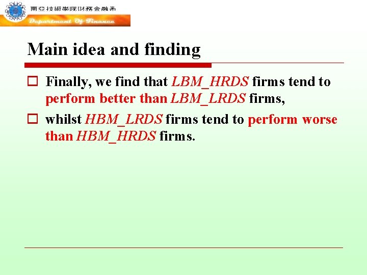
Main idea and finding o Finally, we find that LBM_HRDS firms tend to perform better than LBM_LRDS firms, o whilst HBM_LRDS firms tend to perform worse than HBM_HRDS firms.

INTRODUCTION o It is argued in many of the prior studies (such as Fama and French, 1992 and Kothari and Shanken, 1997), that although firms with a high book-to-market (BM) ratio invariably tend to exhibit poor prior performance, they also exhibit high future returns.

INTRODUCTION o Empirical evidence on this positive BM-returns relationship has been widely documented; Examples include Chan et al. (1991), Daniel and Titman (1997), Fama and French (1998), Elfakhani, Lockwoord and Zaher (1998) and Chiao and Hueng (2005). o however, there are some who challenge this accepted theory.

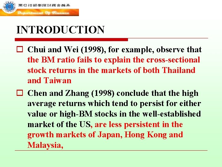
INTRODUCTION o Chui and Wei (1998), for example, observe that the BM ratio fails to explain the cross-sectional stock returns in the markets of both Thailand Taiwan o Chen and Zhang (1998) conclude that the high average returns which tend to persist for either value or high-BM stocks in the well-established market of the US, are less persistent in the growth markets of Japan, Hong Kong and Malaysia,

INTRODUCTION o and virtually non-existent in the high-growth markets of Thailand Taiwan. They argue that in Thailand Taiwan, value stocks do not behave like ‘fallen angels’ at all, but rather, that they yield both prior and future positive excess returns.

o The interpretations of the positive BM-returns relationship in the extant literature can be roughly divided into three schools. o the first of which provides support for the riskbased explanation; that is, firms with a high BM ratio tend to have high underlying risks. Examples include Fama and French (1993).

o The second school is based on stock characteristics, with Daniel and Titman (1997) noting that expected stock returns are directly related to stock characteristics, such as the BM ratio and firm size, as opposed to the associated risks (Fama and French, 1992).

o The third school relates to overreaction or excess expectations with regard to the performance of a firm. Lakonishok, Shleifer and Vishny (1994) argue that firms with a high (low) BM ratio may yield higher (lower) returns;

o however, this runs contrary to the argument that naïve investors extrapolate prior earnings growth rates too far into the future, with the result that the market undervalues distressed stocks whilst overvaluing growth stocks. o When these pricing errors are corrected, distressed (or value) stocks have high returns, whilst growth stocks have low returns. Subsequent overreaction then leads to the BM effect.

o The prior studies often examine the source of the BM effect by applying datasets in which the BM premium has been justified; o however, to the best of our knowledge, no study has yet provided any in-depth exploration of how and why the BM effect may be absent. We therefore set out to examine this issue in the present study using the same data which has already been widely used to demonstrate the non-existence of the BM effect in the Taiwan stock market.

Why not Thailand stock market? o We are unable to examine value premiums conditional on R&D intensity in Thailand since most Thai firms do not produce data on R&D expenditure.

DATA o Accounting data and monthly stock returns were obtained from the Taiwan Economic Journal (TEJ) databank on all non-financial listed firms. o The annual accounting data, covering the years 1991 to 2006, provides a total of 6, 494 firm-year observations, whilst the monthly stock returns, which are available from July 1992 to June 2008, provide a maximum of 192 monthly observations for each stock.

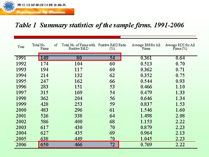
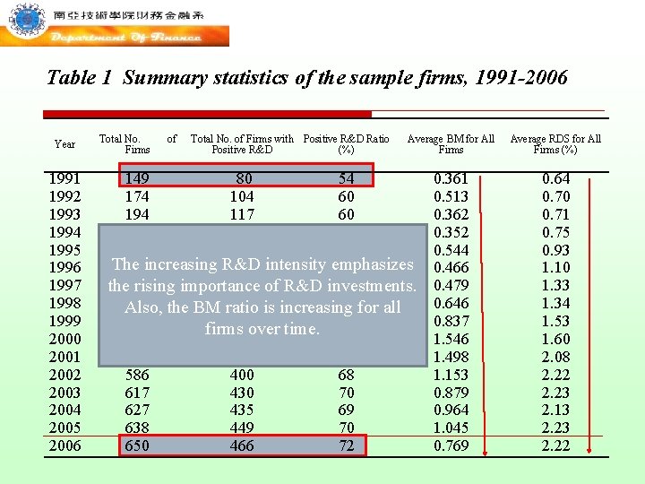
Table 1 Summary statistics of the sample firms, 1991 -2006 Year 1991 1992 1993 1994 1995 1996 1997 1998 1999 2000 2001 2002 2003 2004 2005 2006 Total No. Firms 149 174 194 214 247 283 315 362 428 483 526 586 617 627 638 650 of Total No. of Firms with Positive R&D Ratio Positive R&D (%) 80 104 117 132 162 151 169 204 253 296 338 400 435 449 466 54 60 60 62 66 53 54 56 59 61 64 68 70 69 70 72 Average BM for All Firms Average RDS for All Firms (%) 0. 361 0. 513 0. 362 0. 352 0. 544 0. 466 0. 479 0. 646 0. 837 1. 546 1. 498 1. 153 0. 879 0. 964 1. 045 0. 769 0. 64 0. 70 0. 71 0. 75 0. 93 1. 10 1. 33 1. 34 1. 53 1. 60 2. 08 2. 22 2. 23 2. 13 2. 22

Table 1 Summary statistics of the sample firms, 1991 -2006 Year 1991 1992 1993 1994 1995 1996 1997 1998 1999 2000 2001 2002 2003 2004 2005 2006 Total No. Firms of Total No. of Firms with Positive R&D Ratio Positive R&D (%) Average BM for All Firms 149 80 54 174 104 60 194 117 60 214 132 62 247 162 66 The 283 increasing R&D 151 intensity emphasizes 53 169 of R&D investments. 54 the 315 rising importance 362 the BM ratio 204 is increasing 56 for all Also, 428 253 over time. 59 firms 483 296 61 526 338 64 586 400 68 617 430 70 627 435 69 638 449 70 650 466 72 0. 361 0. 513 0. 362 0. 352 0. 544 0. 466 0. 479 0. 646 0. 837 1. 546 1. 498 1. 153 0. 879 0. 964 1. 045 0. 769 Average RDS for All Firms (%) 0. 64 0. 70 0. 71 0. 75 0. 93 1. 10 1. 33 1. 34 1. 53 1. 60 2. 08 2. 22 2. 23 2. 13 2. 22

2. 2 Portfolio Analysis o We carry out portfolio analyses of the full sample and sub-samples of firms to closely examine the existence of the BM effect in the Taiwan stock market, with the BM-based portfolios. o At the beginning of each July from 1992 to 2008, each stock in a given sample is assigned to one of five portfolios based on its BM ratio. Stocks with a non-positive book value are excluded for the formation date in that year.

o Portfolio ‘Low’ (‘High’) refers to the portfolio with the lowest (highest) BM ratio. ‘H-L’ denotes a zero-investment portfolio formed by buying the portfolio with the highest BM ratio and short-selling the portfolio with the lowest BM ratio. We then calculate the equallyweighted monthly returns.

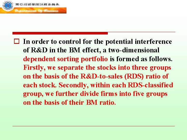
o In order to control for the potential interference of R&D in the BM effect, a two-dimensional dependent sorting portfolio is formed as follows. Firstly, we separate the stocks into three groups on the basis of the R&D-to-sales (RDS) ratio of each stock. Secondly, within each RDS-classified group, we further divide firms into five groups on the basis of their BM ratio.

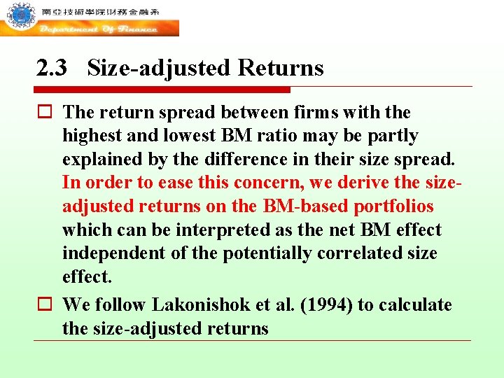
2. 3 Size-adjusted Returns o The return spread between firms with the highest and lowest BM ratio may be partly explained by the difference in their size spread. In order to ease this concern, we derive the sizeadjusted returns on the BM-based portfolios which can be interpreted as the net BM effect independent of the potentially correlated size effect. o We follow Lakonishok et al. (1994) to calculate the size-adjusted returns

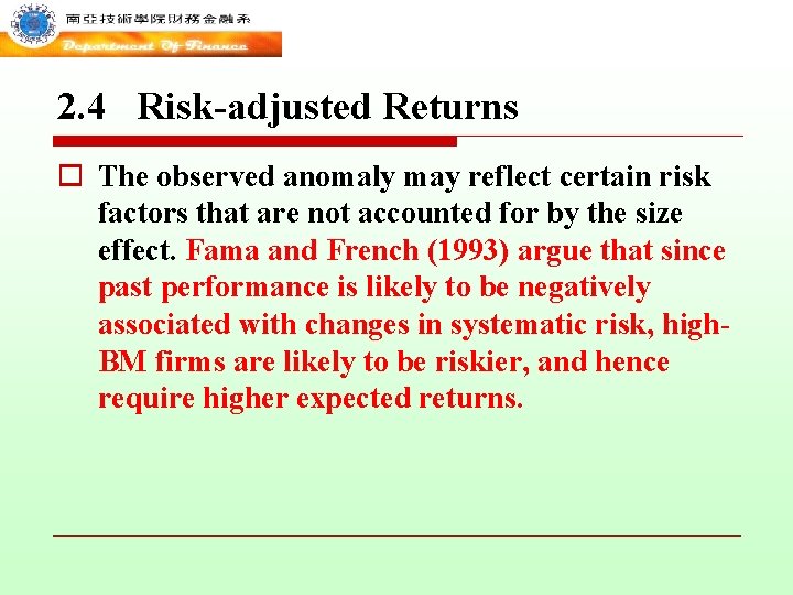
2. 4 Risk-adjusted Returns o The observed anomaly may reflect certain risk factors that are not accounted for by the size effect. Fama and French (1993) argue that since past performance is likely to be negatively associated with changes in systematic risk, high. BM firms are likely to be riskier, and hence require higher expected returns.

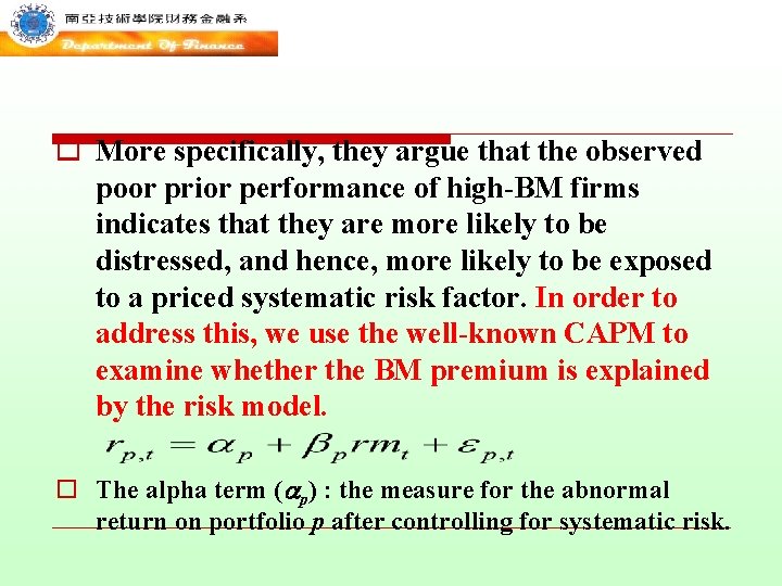
o More specifically, they argue that the observed poor prior performance of high-BM firms indicates that they are more likely to be distressed, and hence, more likely to be exposed to a priced systematic risk factor. In order to address this, we use the well-known CAPM to examine whether the BM premium is explained by the risk model. o The alpha term ( p) : the measure for the abnormal return on portfolio p after controlling for systematic risk.

2. 5 Reversal Coefficient o Lakonishok et al. (1994) argue that investors will often tend to extrapolate the prior performance of a firm to assess its future performance, since they tend to overestimate the performance of growth (low-BM) stocks which have done well in the past, and underestimate the performance of value (high-BM) stocks that have done poorly.

o Thus, they are invariably disappointed (positively surprised) by the growth (value) stocks, as compared to their initial expectations. The BM effect may therefore reflect the overreaction of investors to prior performance. In order to precisely measure the observed magnitude of fundamental reversals, we construct the following simple ex-post index:

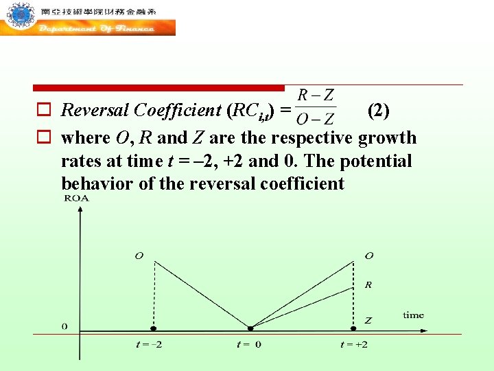
o Reversal Coefficient (RCi, t) = (2) o where O, R and Z are the respective growth rates at time t = – 2, +2 and 0. The potential behavior of the reversal coefficient

o We use the return on assets (ROA) and the return on equity (ROE) in this study as proxies for the profitability of the firm, which is assumed to follow a mean-reversion process. The reversal coefficient (RCi, t) for firm i at time t can therefore be interpreted as follows

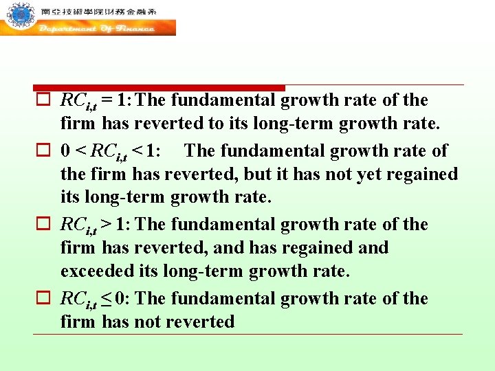
o RCi, t = 1: The fundamental growth rate of the firm has reverted to its long-term growth rate. o 0 < RCi, t < 1: The fundamental growth rate of the firm has reverted, but it has not yet regained its long-term growth rate. o RCi, t > 1: The fundamental growth rate of the firm has reverted, and has regained and exceeded its long-term growth rate. o RCi, t ≤ 0: The fundamental growth rate of the firm has not reverted

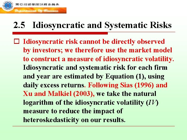
2. 5 Idiosyncratic and Systematic Risks o Idiosyncratic risk cannot be directly observed by investors; we therefore use the market model to construct a measure of idiosyncratic volatility. Idiosyncratic and systematic risk for each firm and year are estimated by Equation (1), using daily excess returns. Following Sias (1996) and Xu and Malkiel (2003), we take the natural logarithm of the idiosyncratic volatility (IV) measure to reduce the impact of heteroskedasticity on our results.

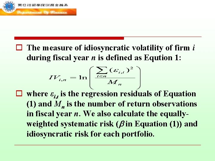
o The measure of idiosyncratic volatility of firm i during fiscal year n is defined as Eqution 1: o where εi, t is the regression residuals of Equation (1) and Mn is the number of return observations in fiscal year n. We also calculate the equallyweighted systematic risk ( in Equation (1)) and idiosyncratic risk for each portfolio.

the BM effect is generally absent in the Taiwan stock market Table 2 Average monthly returns on the book-tomarket based portfolios Book-to-market portfolios Low 2 3 4 High Panel A: Average Raw Monthly Returns (%) Returns 0. 49 0. 73 0. 75 0. 92 1. 49* t-value 0. 75 1. 21 1. 28 1. 45 1. 86 Panel B: Size-adjusted Monthly Returns (%) Returns – 0. 22 – 0. 04 – 0. 13 – 0. 07 0. 44 t-value – 0. 97 – 0. 28 – 1. 21 – 0. 49 1. 59 Panel C: CAPM Risk-adjusted Returns (%) Jensen’s – 0. 16 0. 07 0. 13 0. 34 0. 77 t-value – 0. 49 0. 24 0. 43 0. 93 1. 26 Panel D: Characteristics 0. 298 0. 487 0. 687 0. 953 1. 550 BM 0. 026 0. 020 0. 014 0. 007 0. 005 RDS 7. 141 7. 253 6. 979 7. 029 6. 723 ln(ME) 0. 943 0. 885 0. 844 0. 863 0. 983 Beta S. D. 8. 963 8. 374 8. 137 8. 803 11. 079 Variables H-L 1. 00 1. 50 0. 67 1. 43 0. 93 1. 40 1. 252 – 0. 021 – 0. 417 0. 040 2. 116

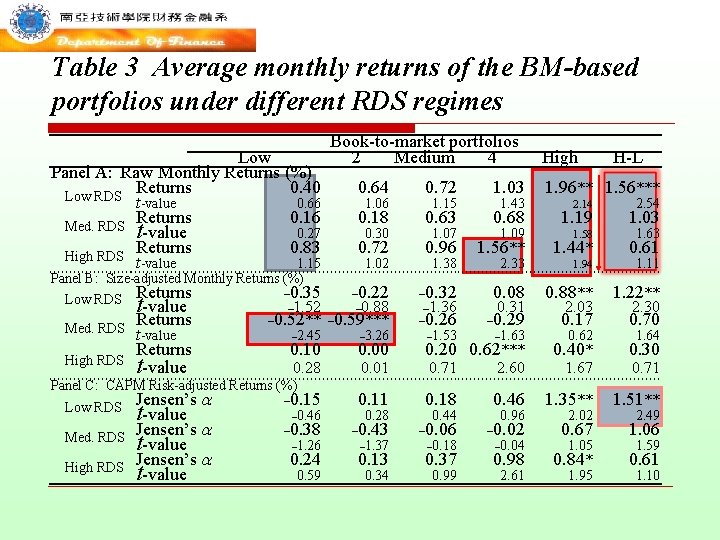
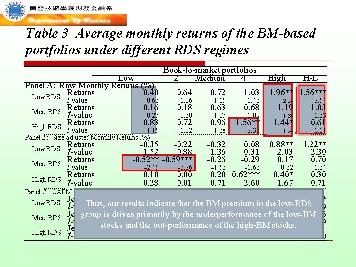
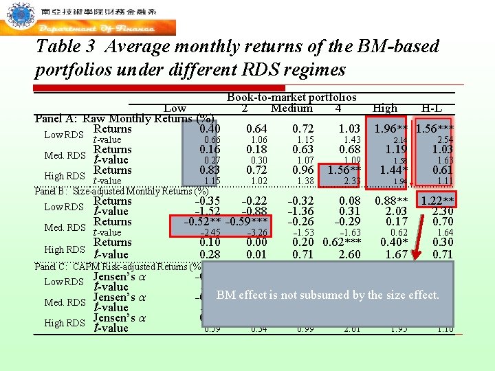
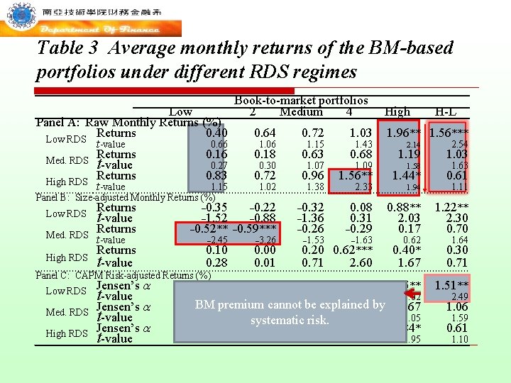
Table 3 Average monthly returns of the BM-based portfolios under different RDS regimes Low Panel A: Raw Monthly Returns (%) Returns 0. 40 Low RDS t-value 0. 66 Returns 0. 16 Med. RDS t-value 0. 27 Returns 0. 83 High RDS t-value 1. 15 Med. RDS High RDS Returns t-value Med. RDS High RDS Jensen’s t-value 0. 72 1. 03 0. 18 0. 63 0. 68 1. 06 0. 30 0. 72 1. 07 0. 96 1. 38 1. 43 1. 09 1. 56** 2. 14 1. 19 1. 58 1. 44* 2. 54 1. 03 1. 63 0. 61 0. 88** 2. 03 0. 17 1. 22** 2. 30 0. 70 0. 00 0. 20 0. 62*** 0. 71 2. 60 0. 40* 0. 30 – 0. 15 0. 11 0. 18 0. 46 1. 35** 1. 51** – 0. 38 – 0. 43 – 0. 06 – 0. 02 0. 67 1. 06 0. 24 0. 13 0. 37 0. 98 0. 84* 0. 61 – 0. 22 – 0. 32 – 0. 52** – 0. 59*** – 0. 26 – 1. 52 – 2. 45 0. 10 0. 28 – 0. 46 – 1. 26 0. 59 – 0. 88 – 3. 26 0. 01 0. 28 – 1. 37 0. 34 – 1. 36 – 1. 53 0. 44 – 0. 18 0. 99 2. 33 1. 96** 1. 56*** 0. 08 0. 31 – 0. 29 – 0. 35 1. 02 1. 15 H-L 1. 11 Panel C: CAPM Risk-adjusted Returns (%) Low RDS 0. 64 High 1. 94 Panel B: Size-adjusted Monthly Returns (%) Low RDS Book-to-market portfolios 2 Medium 4 – 1. 63 0. 96 – 0. 04 2. 61 0. 62 1. 67 2. 02 1. 05 1. 95 1. 64 0. 71 2. 49 1. 59 1. 10

Table 3 Average monthly returns of the BM-based portfolios under different RDS regimes Low Panel A: Raw Monthly Returns (%) Returns 0. 40 Low RDS t-value 0. 66 Returns 0. 16 Med. RDS t-value 0. 27 Returns 0. 83 High RDS t-value 1. 15 Panel B: Size-adjusted Monthly Returns (%) Low RDS Med. RDS High RDS Returns t-value Med. RDS High RDS 0. 64 0. 72 1. 03 0. 18 0. 63 0. 68 1. 06 0. 30 0. 72 1. 02 – 0. 35 – 1. 52 – 0. 22 – 0. 88 – 2. 45 – 3. 26 – 0. 52** – 0. 59*** 0. 10 0. 28 Panel C: CAPM Risk-adjusted Returns (%) Low RDS Book-to-market portfolios 2 Medium 4 0. 00 0. 01 1. 15 1. 07 0. 96 1. 38 1. 43 1. 09 1. 56** H-L 1. 96** 1. 56*** 2. 14 1. 19 1. 58 1. 44* 2. 54 1. 03 1. 63 0. 61 1. 94 1. 11 0. 08 0. 31 – 0. 29 0. 88** 2. 03 0. 17 1. 22** 2. 30 0. 70 0. 20 0. 62*** 0. 71 2. 60 0. 40* 1. 67 0. 30 0. 71 – 0. 32 – 1. 36 – 0. 26 – 1. 53 2. 33 High – 1. 63 0. 62 1. 64 Jensen’s – 0. 15 0. 11 0. 18 0. 46 1. 35** 1. 51** Thus, our results indicate that the BM premium t-value – 0. 46 0. 28 0. 44 0. 96 in the low-RDS 2. 02 2. 49 Jensen’s – 0. 38 – 0. 43 – 0. 06 – 0. 02 of the 0. 67 1. 06 group is driven primarily by the underperformance low-BM t-value stocks and the – 1. 26 – 1. 37 – 0. 18 – 0. 04 1. 05 1. 59 out-performance of the high-BM Jensen’s 0. 24 0. 13 0. 37 0. 98 stocks. 0. 84* 0. 61 t-value 0. 59 0. 34 0. 99 2. 61 1. 95 1. 10

Table 3 Average monthly returns of the BM-based portfolios under different RDS regimes Low Panel A: Raw Monthly Returns (%) Returns 0. 40 Low RDS t-value 0. 66 Returns 0. 16 Med. RDS t-value 0. 27 Returns 0. 83 High RDS t-value 1. 15 Panel B: Size-adjusted Monthly Returns (%) Low RDS Med. RDS High RDS Returns t-value Book-to-market portfolios 2 Medium 4 0. 64 0. 72 1. 03 0. 18 0. 63 0. 68 1. 06 0. 30 0. 72 1. 02 – 0. 35 – 1. 52 – 0. 22 – 0. 88 – 2. 45 – 3. 26 – 0. 52** – 0. 59*** 0. 10 0. 28 0. 00 0. 01 1. 15 1. 07 0. 96 1. 38 1. 43 1. 09 1. 56** H-L 1. 96** 1. 56*** 2. 14 1. 19 1. 58 1. 44* 2. 54 1. 03 1. 63 0. 61 1. 94 1. 11 0. 08 0. 31 – 0. 29 0. 88** 2. 03 0. 17 1. 22** 2. 30 0. 70 0. 20 0. 62*** 0. 71 2. 60 0. 40* 1. 67 0. 30 0. 71 – 0. 32 – 1. 36 – 0. 26 – 1. 53 2. 33 High – 1. 63 0. 62 1. 64 Panel C: CAPM Risk-adjusted Returns (%) Low RDS Med. RDS High RDS Jensen’s t-value – 0. 15 0. 11 0. 18 0. 46 1. 35** 1. 51** – 0. 46 0. 28 0. 44 0. 96 2. 02 2. 49 BM effect is not subsumed by the size effect. – 0. 38 – 0. 43 – 0. 06 – 0. 02 0. 67 1. 06 – 1. 26 0. 24 0. 59 – 1. 37 0. 13 0. 34 – 0. 18 0. 37 0. 99 – 0. 04 0. 98 2. 61 1. 05 0. 84* 1. 95 1. 59 0. 61 1. 10

Table 3 Average monthly returns of the BM-based portfolios under different RDS regimes Low Panel A: Raw Monthly Returns (%) Returns 0. 40 Low RDS t-value 0. 66 Returns 0. 16 Med. RDS t-value 0. 27 Returns 0. 83 High RDS t-value 1. 15 Med. RDS High RDS Returns t-value Med. RDS High RDS Jensen’s t-value 0. 72 1. 03 0. 18 0. 63 0. 68 1. 06 0. 30 0. 72 1. 02 1. 15 1. 07 0. 96 1. 09 1. 56** 2. 14 1. 19 1. 58 1. 44* 2. 54 1. 03 1. 63 0. 61 0. 88** 2. 03 0. 17 1. 22** 2. 30 0. 70 0. 01 0. 20 0. 62*** 0. 71 2. 60 0. 40* 1. 67 0. 30 0. 71 0. 18 1. 35** 1. 51** BM premium cannot– 0. 06 be explained – 0. 38 – 0. 43 – 0. 02 by 0. 67 – 1. 26 – 1. 37 – 0. 18 – 0. 04 1. 05 systematic risk. 0. 24 0. 13 0. 37 0. 98 0. 84* 1. 06 – 0. 22 – 0. 88 – 2. 45 – 3. 26 – 0. 52** – 0. 59*** 0. 10 0. 28 – 0. 15 – 0. 46 0. 59 0. 28 0. 34 – 0. 32 – 1. 36 – 0. 26 – 1. 53 0. 44 0. 99 2. 33 1. 96** 1. 56*** 0. 08 0. 31 – 0. 29 – 0. 35 – 1. 52 1. 38 1. 43 H-L 1. 11 Panel C: CAPM Risk-adjusted Returns (%) Low RDS 0. 64 High 1. 94 Panel B: Size-adjusted Monthly Returns (%) Low RDS Book-to-market portfolios 2 Medium 4 – 1. 63 0. 46 0. 96 2. 61 0. 62 2. 02 1. 95 1. 64 2. 49 1. 59 0. 61 1. 10

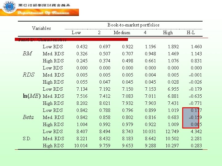
Variables Panel D: Characteristics Low RDS BM Med. RDS High RDS Low RDS ln(ME) Med. RDS High RDS Low RDS Beta Med. RDS High RDS Low RDS S. D. Med. RDS High RDS Book-to-market portfolios Low 0. 432 0. 326 0. 245 0. 000 0. 005 0. 055 7. 134 7. 516 8. 202 0. 842 1. 004 8. 407 8. 221 10. 014 2 0. 697 0. 507 0. 374 0. 000 0. 005 0. 047 7. 192 7. 412 8. 021 0. 788 0. 858 0. 992 8. 494 8. 432 9. 759 Medium 0. 922 0. 707 0. 498 0. 000 0. 005 0. 045 7. 150 7. 083 7. 932 0. 796 0. 802 0. 979 8. 743 8. 183 9. 653 4 1. 196 0. 948 0. 661 0. 000 0. 004 0. 045 7. 153 7. 011 7. 903 0. 899 0. 816 0. 922 10. 031 8. 642 9. 288 High 1. 892 1. 469 1. 076 0. 000 0. 005 0. 028 6. 955 6. 881 7. 431 1. 019 0. 683 1. 009 12. 749 10. 502 10. 297 H-L 1. 460 1. 143 0. 831 0. 000 – 0. 001 – 0. 026 – 0. 179 – 0. 635 – 0. 771 0. 177 – 0. 159 0. 005 4. 342 2. 281 0. 283

Figure 2 Cumulative returns on portfolios sorted by book-tomarket ratio under high- and low-RDS regimes

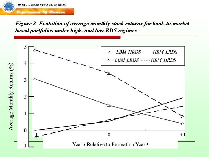
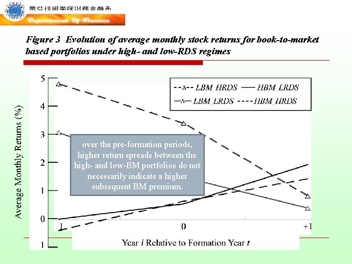
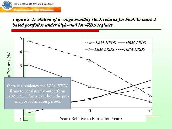
Figure 3 Evolution of average monthly stock returns for book-to-market based portfolios under high- and low-RDS regimes

Figure 3 Evolution of average monthly stock returns for book-to-market based portfolios under high- and low-RDS regimes over the pre-formation periods, higher return spreads between the high- and low-BM portfolios do not necessarily indicate a higher subsequent BM premium.

Figure 3 Evolution of average monthly stock returns for book-to-market based portfolios under high- and low-RDS regimes there is a tendency for LBM_HRDS firms to consistently outperform LBM_LRDS firms over both the preand post-formation periods

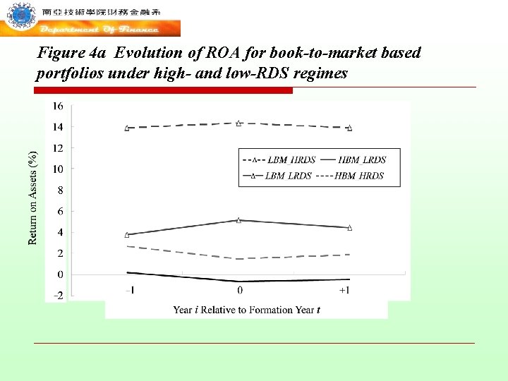
Figure 4 a Evolution of ROA for book-to-market based portfolios under high- and low-RDS regimes

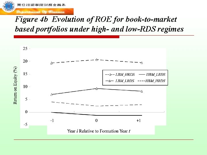
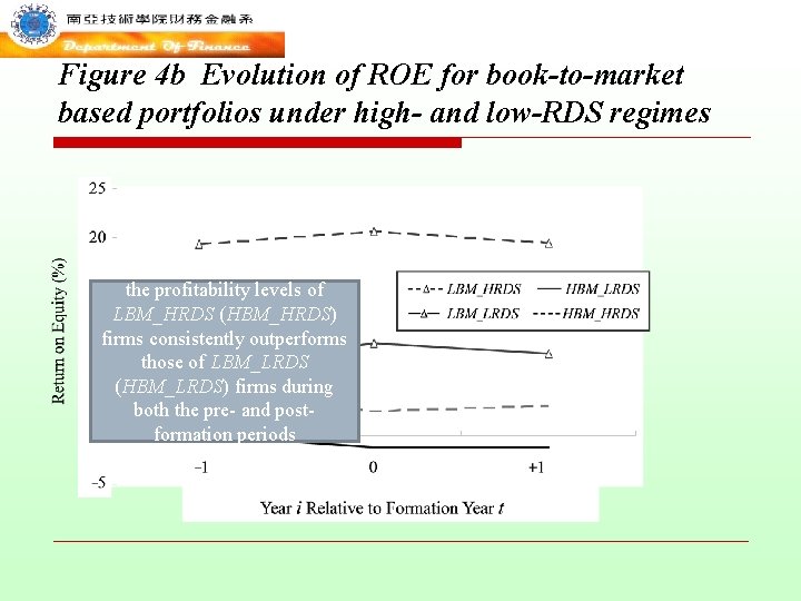
Figure 4 b Evolution of ROE for book-to-market based portfolios under high- and low-RDS regimes

Figure 4 b Evolution of ROE for book-to-market based portfolios under high- and low-RDS regimes the profitability levels of LBM_HRDS (HBM_HRDS) firms consistently outperforms those of LBM_LRDS (HBM_LRDS) firms during both the pre- and postformation periods

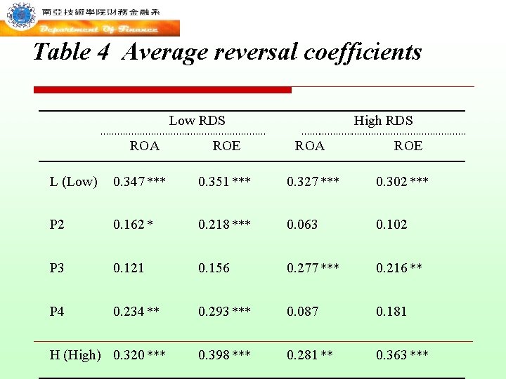
Table 4 Average reversal coefficients Low RDS ROA High RDS ROE ROA ROE L (Low) 0. 347 *** 0. 351 *** 0. 327 *** 0. 302 *** P 2 0. 162 * 0. 218 *** 0. 063 0. 102 P 3 0. 121 0. 156 0. 277 *** 0. 216 ** P 4 0. 234 ** 0. 293 *** 0. 087 0. 181 0. 398 *** 0. 281 ** 0. 363 *** H (High) 0. 320 ***

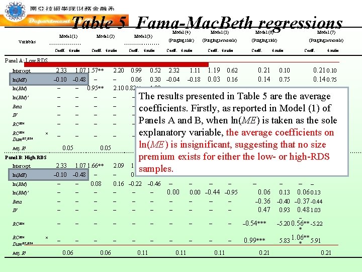
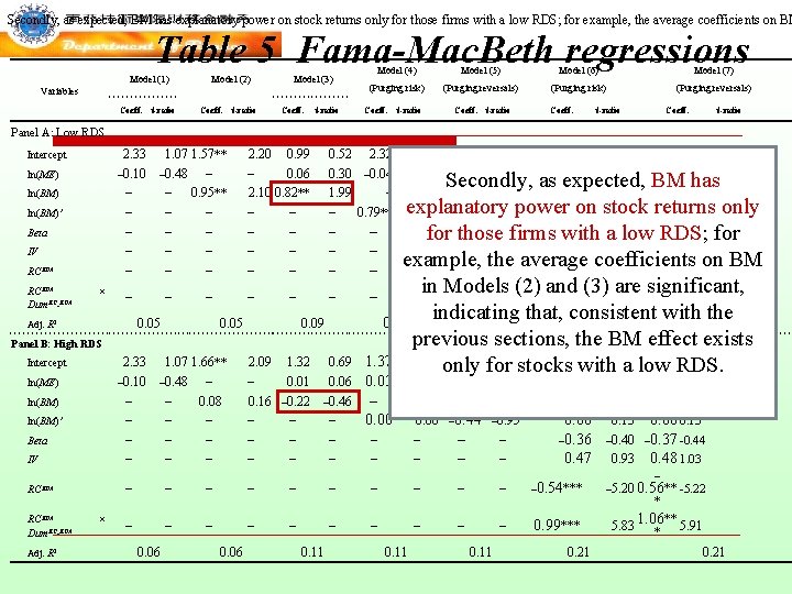
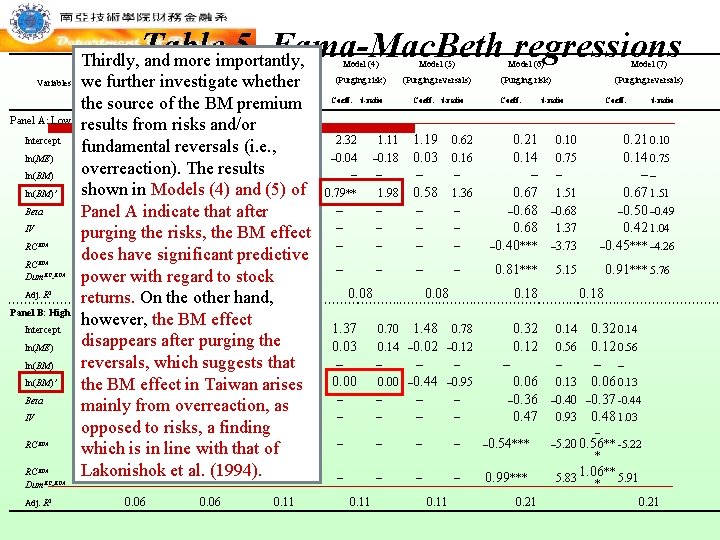
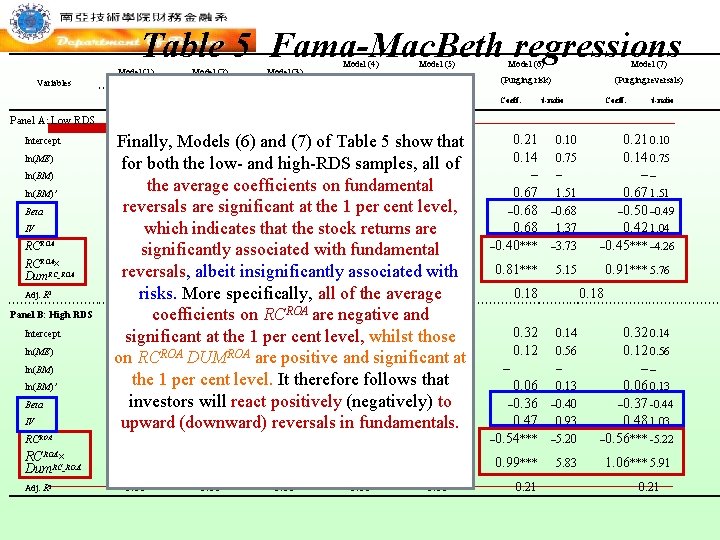
Table 5 Fama-Mac. Beth regressions Model (1) Model (2) Model (3) Variables Coeff. t-ratio Model (4) Model (5) Model (6) Model (7) (Purging risk) (Purging reversals) Coeff. t-ratio Panel A: Low RDS 2. 33 1. 07 1. 57** – 0. 10 – 0. 48 – – – 0. 95** – – – Intercept ln(ME) ln(BM)′ Beta IV RCROA Dum. RC_ROA × – – – 0. 05 Adj. R 2 2. 20 0. 99 – 0. 06 2. 10 0. 82** – – – – 0. 52 2. 32 0. 30 – 0. 04 1. 99 – – 0. 79** – – – – – 0. 05 1. 11 – 0. 18 – 1. 98 – – – 1. 19 0. 03 – 0. 58 – – – 0. 62 0. 16 – 1. 36 – – – – 0. 08 0. 09 0. 21 0. 14 – 0. 67 – 0. 68 – 0. 40*** 0. 10 0. 75 – 1. 51 – 0. 68 1. 37 – 3. 73 0. 21 0. 10 0. 14 0. 75 –– 0. 67 1. 51 – 0. 50 – 0. 49 0. 42 1. 04 – 0. 45*** – 4. 26 0. 81*** 5. 15 0. 91*** 5. 76 0. 08 0. 18 Panel B: High RDS 2. 33 1. 07 1. 66** – 0. 10 – 0. 48 – – – 0. 08 – – – – – Intercept ln(ME) ln(BM)′ Beta IV – RCROA Dum. RC_ROA Adj. R 2 × – – – 0. 06 – 2. 09 1. 32 – 0. 01 0. 16 – 0. 22 – – – – – 0. 06 0. 69 0. 06 – 0. 46 – – – – 0. 11 1. 37 0. 03 – 0. 00 – – 0. 70 1. 48 0. 78 0. 14 – 0. 02 – 0. 12 – – – 0. 00 – 0. 44 – 0. 95 – – – – – 0. 11 0. 32 0. 12 – 0. 06 – 0. 36 0. 47 0. 14 0. 32 0. 14 0. 56 0. 12 0. 56 – – – 0. 13 0. 06 0. 13 – 0. 40 – 0. 37 -0. 44 0. 93 0. 48 1. 03 – 0. 54*** – – 5. 20 0. 56** -5. 22 0. 99*** 1. 06** 5. 91 5. 83 0. 21 * * 0. 21

Table 5 Fama-Mac. Beth regressions Model (1) Model (2) Model (3) Variables Coeff. t-ratio Model (4) Model (5) Model (6) Model (7) (Purging risk) (Purging reversals) Coeff. t-ratio Panel A: Low RDS 2. 33 1. 07 1. 57** – 0. 10 – 0. 48 – – – 0. 95** – – – Intercept ln(ME) ln(BM)′ Beta IV RCROA Dum. RC_ROA × – – – 0. 05 Adj. R 2 1. 19 0. 62 0. 21 0. 10 0. 03 0. 16 0. 14 0. 75 – – –– The results presented 5 are 1. 51 the average 0. 58 in 1. 36 Table 0. 67 1. 51 – as– reported – 0. 68 – 0. 50 – 0. 49 coefficients. Firstly, in Model (1) of – – 0. 68 1. 37 0. 42 1. 04 Panels A and B, when is taken as– 0. 45 the***sole – 4. 26 – –ln(ME) – 0. 40*** – 3. 73 2. 20 0. 99 – 0. 06 2. 10 0. 82** – – – – – 0. 05 Panel B: High RDS 2. 33 1. 07 1. 66** – 0. 10 – 0. 48 – – – 0. 08 – – – – – Intercept ln(ME) ln(BM)′ Beta IV – RCROA Dum. RC_ROA Adj. R 2 × – – – 0. 06 1. 11 – 0. 18 – 1. 98 – – – explanatory variable, the average 5. 76 – – – 0. 81*** coefficients 5. 15 0. 91***on ln(ME) is 0. 08 insignificant, no size 0. 09 0. 08 suggesting 0. 18 that 0. 18 premium exists for either the low- or high-RDS 1. 32 0. 69 1. 37 0. 70 1. 48 0. 78 0. 32 0. 14 samples. – 2. 09 – 0. 01 0. 16 – 0. 22 – – – – 0. 52 2. 32 0. 30 – 0. 04 1. 99 – – 0. 79** – – – 0. 06 – 0. 46 – – – – 0. 11 0. 03 – 0. 00 – – 0. 14 – 0. 02 – 0. 12 – – – 0. 00 – 0. 44 – 0. 95 – – – – – 0. 11 0. 12 – 0. 06 – 0. 36 0. 47 0. 56 0. 12 0. 56 – – – 0. 13 0. 06 0. 13 – 0. 40 – 0. 37 -0. 44 0. 93 0. 48 1. 03 – 0. 54*** – – 5. 20 0. 56** -5. 22 0. 99*** 1. 06** 5. 91 5. 83 0. 21 * * 0. 21

Secondly, as expected, BM has explanatory power on stock returns only for those firms with a low RDS; for example, the average coefficients on BM Table 5 Fama-Mac. Beth regressions Model (1) Model (2) Model (3) Variables Coeff. t-ratio Model (4) Model (5) Model (6) Model (7) (Purging risk) (Purging reversals) Coeff. t-ratio Panel A: Low RDS 2. 33 1. 07 1. 57** – 0. 10 – 0. 48 – – – 0. 95** – – – Intercept ln(ME) ln(BM)′ Beta IV RCROA Dum. RC_ROA × – – – 0. 05 Adj. R 2 2. 20 0. 99 – 0. 06 2. 10 0. 82** – – – – 0. 52 2. 32 0. 30 – 0. 04 1. 99 – – 0. 79** – – – – – 0. 05 0. 09 Panel B: High RDS 2. 33 1. 07 1. 66** – 0. 10 – 0. 48 – – – 0. 08 – – – – – Intercept ln(ME) ln(BM)′ Beta IV – RCROA Dum. RC_ROA Adj. R 2 × – – – 0. 06 – 2. 09 1. 32 – 0. 01 0. 16 – 0. 22 – – – – – 0. 06 0. 69 0. 06 – 0. 46 – – – – 0. 11 1. 19 0. 62 0. 21 0. 10 0. 03 0. 16 0. 14 0. 75 Secondly, as expected, BM has – – –– explanatory on stock returns only 0. 58 1. 36 power 0. 67 1. 51 – 0. 49 0. 68 a – 0. 68 – 0. 50 for –those– firms –with low RDS; – – 0. 68 1. 37 0. 42 1. 04 example, the average coefficients on BM – – – 0. 40*** – 3. 73 – 0. 45*** – 4. 26 1. 11 – 0. 18 – 1. 98 – – – in Models (2) 0. 81 and***(3) 5. 15 are significant, – – 0. 91*** 5. 76 indicating that, 0. 18 consistent with the 0. 08 0. 18 previous sections, the BM effect exists 0. 14 1. 37 0. 70 only 1. 48 for 0. 78 stocks 0. 32 RDS. with 0. 14 a low – – 0. 03 – 0. 00 – – 0. 14 – 0. 02 – 0. 12 – – – 0. 00 – 0. 44 – 0. 95 – – – – – 0. 11 0. 12 – 0. 06 – 0. 36 0. 47 0. 56 0. 12 0. 56 – – – 0. 13 0. 06 0. 13 – 0. 40 – 0. 37 -0. 44 0. 93 0. 48 1. 03 – 0. 54*** – – 5. 20 0. 56** -5. 22 0. 99*** 1. 06** 5. 91 5. 83 0. 21 * * 0. 21

Table 5 Fama-Mac. Beth regressions Thirdly, and more importantly, Model (4) Model (5) Model (1) Model (2) Model (3) (Purging risk) (Purging reversals) Variables we further investigate whether Coeff. t-ratio the source of the BM premium Panel A: Low RDS results from risks and/or Intercept 2. 33 1. 07 1. 57** 2. 20 0. 99 0. 52 2. 32 1. 11 1. 19 0. 62 fundamental reversals (i. e. , ln(ME) – 0. 10 – 0. 48 – – 0. 06 0. 30 – 0. 04 – 0. 18 0. 03 0. 16 overreaction). The results ln(BM) – – 0. 95** 2. 10 0. 82** 1. 99 – – shown ln(BM)′ – in –Models – (4)– and –(5) of – 0. 79** 1. 98 0. 58 1. 36 Beta – – that – after– – – Panel– A indicate IV – – – – purging the risks, the– BM– effect RC – – – – – does have significant predictive RC × – – – – – Dum power with regard to– stock Adj. R 0. 05 hand, 0. 09 0. 08 returns. On the other Panel B: High RDS however, the BM effect Intercept 2. 33 1. 07 1. 66** 2. 09 1. 32 0. 69 1. 37 0. 70 1. 48 0. 78 disappears after purging the ln(ME) – 0. 10 – 0. 48 – – 0. 01 0. 06 0. 03 0. 14 – 0. 02 – 0. 12 reversals, that– 0. 46 – ln(BM) – –which 0. 08 suggests 0. 16 – 0. 22 – – – ln(BM)′ – – – Taiwan – – – 0. 00 – 0. 44 – 0. 95 the BM effect in arises Beta – – – – – mainly from overreaction, as – IV – – – – – opposed to risks, a finding RC – – – which is in line– with– that –of – RC × Lakonishok – – et –al. (1994). – – – – ROA RC_ROA Model (6) Model (7) (Purging risk) (Purging reversals) Coeff. ROA Dum. RC_ROA Adj. R 2 0. 06 0. 11 Coeff. t-ratio 0. 21 0. 14 – 0. 67 – 0. 68 – 0. 40*** 0. 10 0. 75 – 1. 51 – 0. 68 1. 37 – 3. 73 0. 21 0. 10 0. 14 0. 75 –– 0. 67 1. 51 – 0. 50 – 0. 49 0. 42 1. 04 – 0. 45*** – 4. 26 0. 81*** 5. 15 0. 91*** 5. 76 0. 18 2 ROA t-ratio 0. 32 0. 12 – 0. 06 – 0. 36 0. 47 0. 18 0. 14 0. 32 0. 14 0. 56 0. 12 0. 56 – – – 0. 13 0. 06 0. 13 – 0. 40 – 0. 37 -0. 44 0. 93 0. 48 1. 03 – 0. 54*** – – 5. 20 0. 56** -5. 22 0. 99*** 1. 06** 5. 91 5. 83 0. 21 * * 0. 21

Table 5 Fama-Mac. Beth regressions Model (1) Model (2) Model (3) Variables Coeff. t-ratio Model (4) Model (5) Model (6) Model (7) (Purging risk) (Purging reversals) Coeff. t-ratio Panel A: Low RDS Intercept ln(ME) ln(BM)′ Beta IV RCROA× Dum. RC_ROA Adj. R 2 Panel B: High RDS Intercept ln(ME) ln(BM) 2. 33 1. 07 1. 57 ** 2. 20 0. 99 (7) 0. 52 of 2. 32 1. 19 that 0. 62 Finally, Models (6) and Table 1. 11 5 show – 0. 10 – 0. 48 – – 0. 06 0. 30 – 0. 04 – 0. 18 0. 03 0. 16 for both the lowand high-RDS samples, all of – – 0. 95** 2. 10 0. 82** 1. 99 – – the average coefficients on fundamental – – – 0. 79** 1. 98 0. 58 1. 36 at – reversals – –are significant – – – the– 1 per– cent –level, – –indicates – – – stock – returns – – – which that the are – – associated – – with – fundamental – – – significantly – reversals, – – albeit – – associated – – with– insignificantly 0. 05 specifically, 0. 09 0. 08 risks. More all of 0. 08 the average coefficients on RCROA are negative and 2. 33 1. 07 1. 66**at the 2. 09 1 1. 32 0. 69 level, 1. 37 whilst 0. 70 1. 48 significant per cent those 0. 78 – 0. 10 – 0. 48 – –ROA 0. 01 0. 06 0. 03 0. 14 – 0. 02 – 0. 12 on RCROA DUM are positive and significant at – – 0. 08 0. 16 – 0. 22 – 0. 46 – – the 1 per cent level. It therefore follows that – – – 0. 00 – 0. 44 – 0. 95 – investors – – will–react– positively – – (negatively) – – to – – upward – – reversals – –in fundamentals. – – – (downward) 0. 21 0. 14 – 0. 67 – 0. 68 – 0. 40*** 0. 10 0. 75 – 1. 51 – 0. 68 1. 37 – 3. 73 0. 21 0. 10 0. 14 0. 75 –– 0. 67 1. 51 – 0. 50 – 0. 49 0. 42 1. 04 – 0. 45*** – 4. 26 0. 81*** 5. 15 0. 91*** 5. 76 0. 18 0. 32 0. 12 – RCROA – – – – – 0. 06 – 0. 36 0. 47 – 0. 54*** RCROA× Dum. RC_ROA – – – – – 0. 99*** ln(BM)′ Beta IV Adj. R 2 0. 06 0. 11 0. 21 0. 18 0. 14 0. 56 – 0. 13 – 0. 40 0. 93 – 5. 20 0. 32 0. 14 0. 12 0. 56 –– 0. 06 0. 13 – 0. 37 -0. 44 0. 48 1. 03 – 0. 56*** -5. 22 5. 83 1. 06*** 5. 91 0. 21

o Thanks for your listening!