Rational consumer choice ECO 61 Microeconomic Analysis Udayan

Rational consumer choice ECO 61 Microeconomic Analysis Udayan Roy Fall 2008

Consumer Choice • We have seen how the consumer’s preferences are represented • And how the consumer’s budget constraint is represented • Now it’s time to bring preferences and constraints together to ask the consumer: • What’s your choice? How do you decide what to buy?

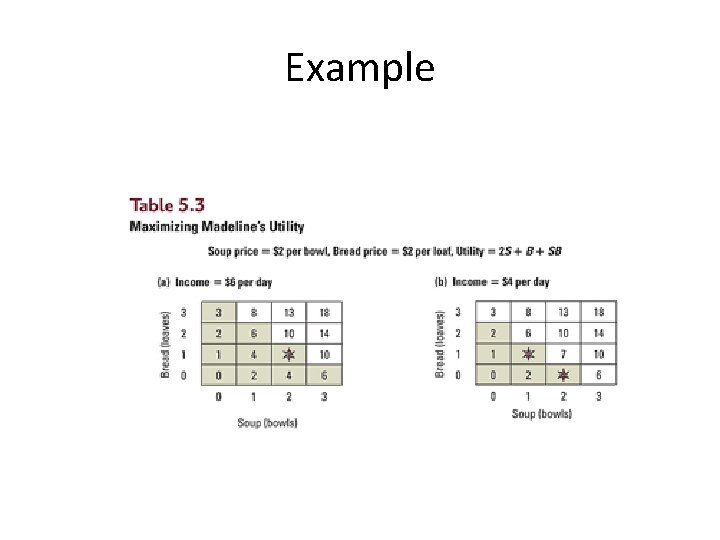
Example

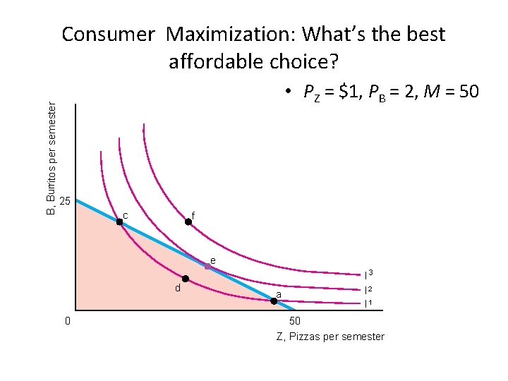
B, Burritos per semester Consumer Maximization: What’s the best affordable choice? • PZ = $1, PB = 2, M = 50 25 c f e d 0 a I 3 I 2 I 1 50 Z, Pizzas per semester

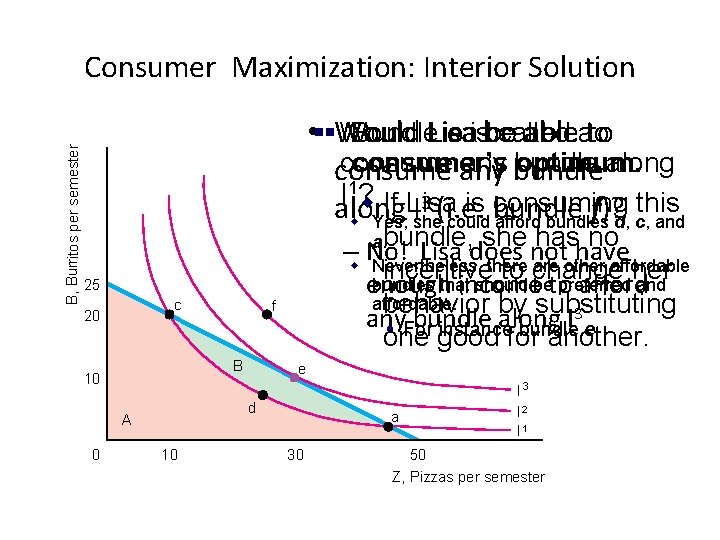
B, Burritos per semester Consumer Maximization: Interior Solution • §§Would Lisa ableato to Would Bundle. Lisa e isbe called consumer’s any bundle optimum. along consume any I 1? w If Lisa 3 (i. e. is bundle consuming this along I f)? w Yes; she could afford bundles d, c, and a. bundle, she has no –w No! Lisa does not have Nevertheless, there are other affordable incentive to change her bundles that should be preferred enough income to affordand affordable. behavior by substituting 3 any bundle along I For good instancefor bundle e one another. 25 c 20 B 10 e d A 0 f 10 a 30 I 3 I 2 I 1 50 Z, Pizzas per semester

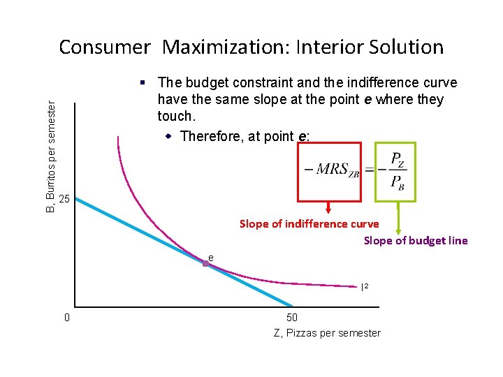
B, Burritos per semester Consumer Maximization: Interior Solution § The budget constraint and the indifference curve have the same slope at the point e where they touch. w Therefore, at point e: 25 Slope of indifference curve Slope of budget line e I 2 0 50 Z, Pizzas per semester

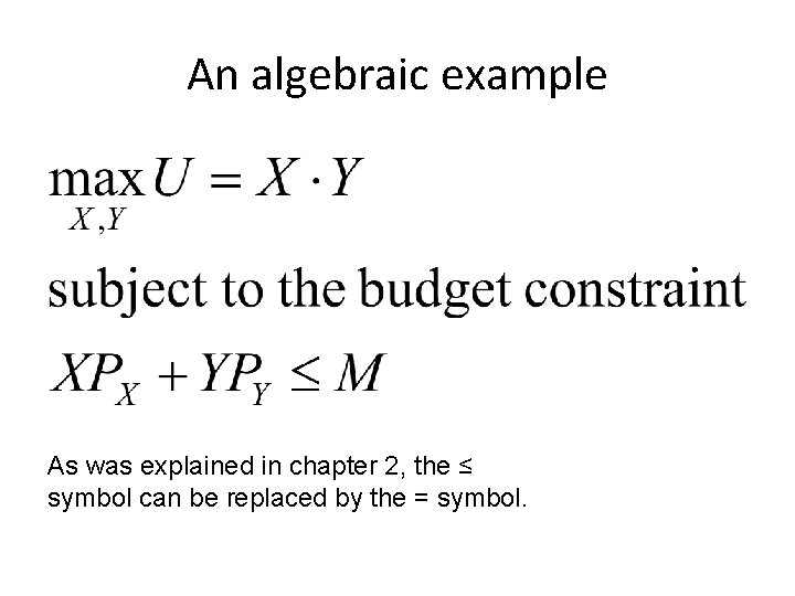
An algebraic example As was explained in chapter 2, the ≤ symbol can be replaced by the = symbol.

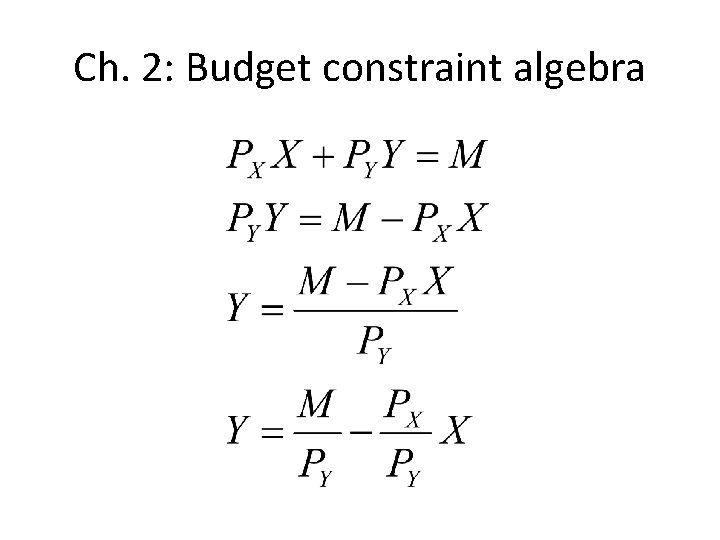
Ch. 2: Budget constraint algebra

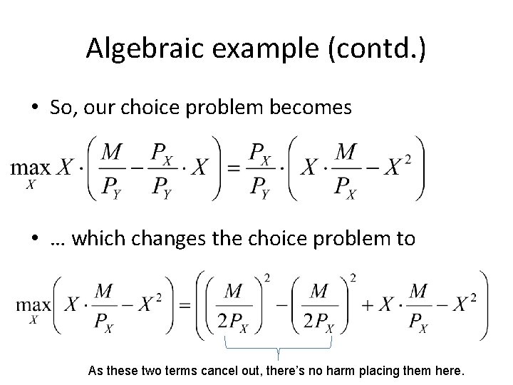
Algebraic example (contd. ) • So, our choice problem becomes • … which changes the choice problem to As these two terms cancel out, there’s no harm placing them here.

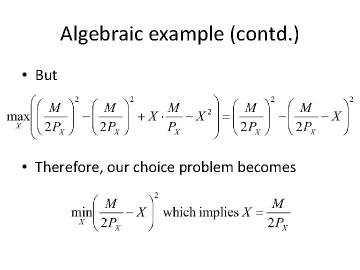
Algebraic example (contd. ) • But • Therefore, our choice problem becomes

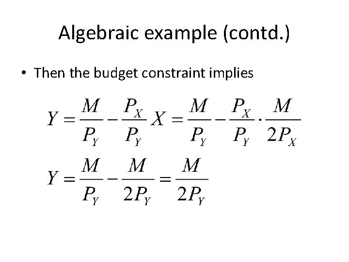
Algebraic example (contd. ) • Then the budget constraint implies

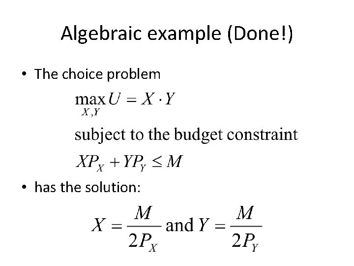
Algebraic example (Done!) • The choice problem • has the solution:

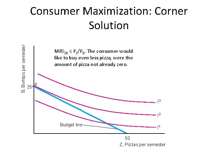
B, Burritos per semester Consumer Maximization: Corner Solution MRSZB ≤ PZ/PB. The consumer would like to buy even less pizza, were the amount of pizza not already zero. 25 e I 3 I 2 Budget line I 1 50 Z, Pizzas per semester

Food Stamps • Nearly 11% of U. S. households worry about having enough money to buy food and 3. 3% report that they suffer from inadequate food. • Households that meet income, asset, and employment eligibility requirements receive coupons that can be used to purchase food from retail stores.

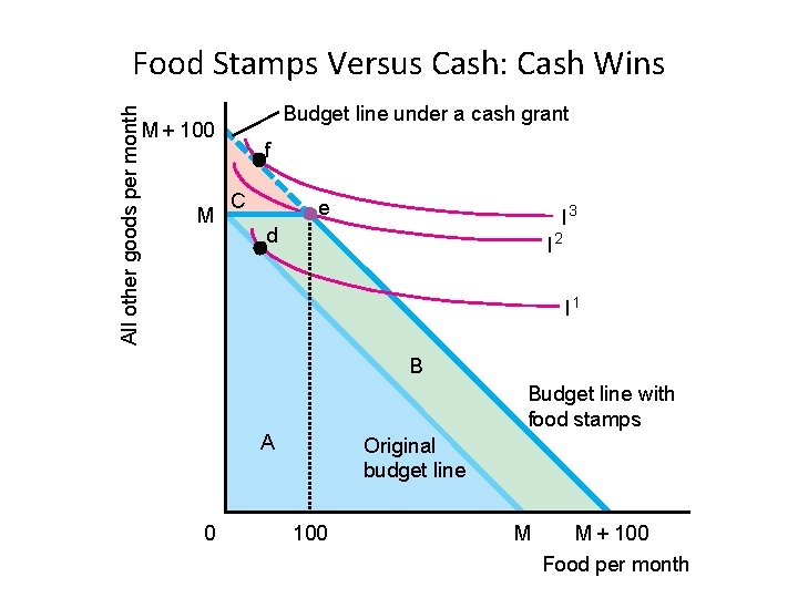
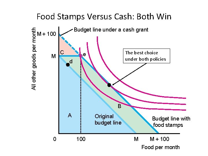
Food Stamps (cont). • The Food Stamps Program is one of the nation’s largest social welfare programs with expenditures of $33. 1 billion for nearly 29. 1 million people in 2006. • Would a switch to a comparable cash subsidy increase the well-being of food stamp recipients? – Would the recipients spend less on food and more on other goods?

All other goods per month Food Stamps Versus Cash: Cash Wins Budget line under a cash grant M + 100 M f C e I 3 d I 2 I 1 B Budget line with food stamps A 0 Original budget line 100 M M + 100 Food per month

All other goods per month Food Stamps Versus Cash: Both Win Budget line under a cash grant M + 100 M C The best choice under both policies e d B A 0 Original budget line 100 Budget line with food stamps M M + 100 Food per month

Gifts: cash or kind? • In the hit TV show Seinfeld, Elaine was once furious when Jerry gave her cash as a birthday gift – She was not objecting to the amount, which was $182 • Does Jerry deserve such harsh treatment?

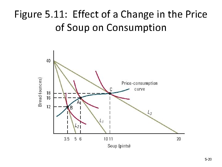
Figure 5. 11: Effect of a Change in the Price of Soup on Consumption 5 -20

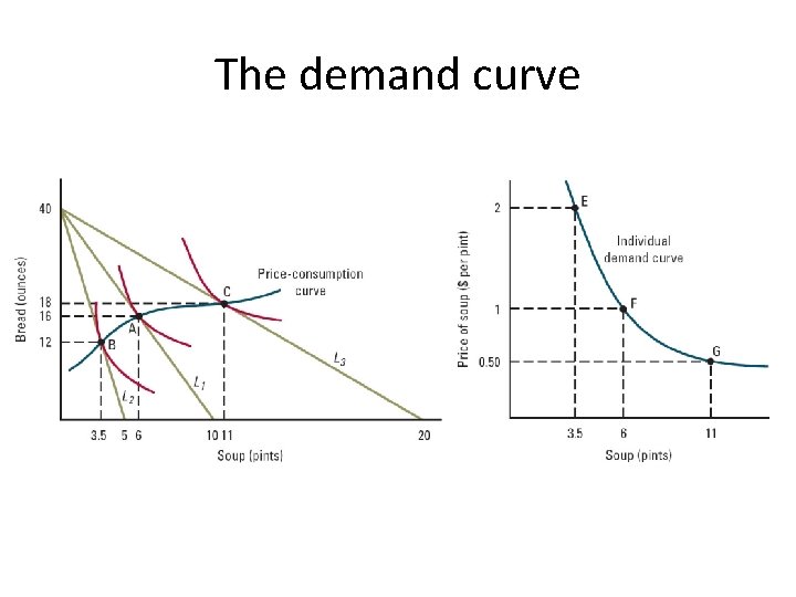
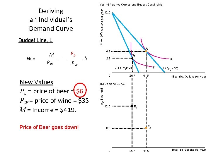
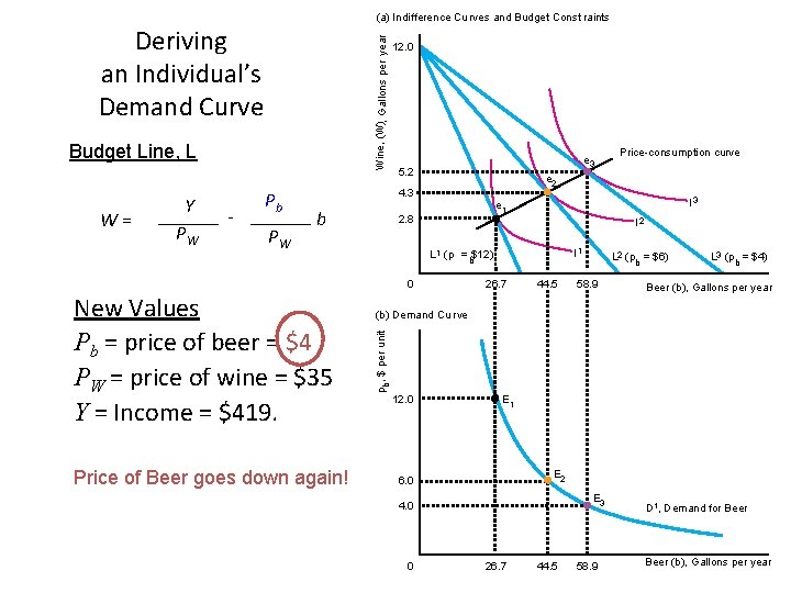
The demand curve

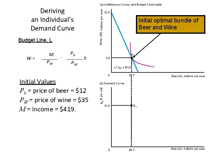
(a) Indifference Cu rves and Budget Const raints Wine, (W), Gallons per year Deriving an Individual’s Demand Curve Budget Line, L W= M PW - Pb PW b 12. 0 Initial optimal bundle of Beer and Wine e 1 2. 8 0 26. 7 Beer (b), Gallons per year (b) Demand Cu rve pb, $ per unit Initial Values Pb = price of beer = $12 PW = price of wine = $35 M = Income = $419. I 1 L 1 (pb = $12) 12. 0 0 E 1 26. 7 Beer (b), Gallons per year

(a) Indifference Cu rves and Budget Const raints Wine, (W), Gallons per year Deriving an Individual’s Demand Curve Budget Line, L W= M PW - Pb PW 12. 0 e 2 4. 3 b e 1 2. 8 I 2 0 Price of Beer goes down! 26. 7 44. 5 L 2 (pb = $6) Beer (b), Gallons per year (b) Demand Cu rve pb, $ per unit New Values Pb = price of beer = $6 PW = price of wine = $35 M = Income = $419. I 1 L 1 (p = b$12) 12. 0 E 1 E 2 6. 0 0 26. 7 44. 5 Beer (b), Gallons per year

(a) Indifference Cu rves and Budget Const raints Wine, (W), Gallons per year Deriving an Individual’s Demand Curve Budget Line, L W= Y PW - Pb PW 12. 0 e 3 5. 2 e 2 4. 3 b Price of Beer goes down again! I 3 e 1 2. 8 I 2 I 1 L 1 (p = b$12) 0 26. 7 44. 5 L 2 (pb = $6) 58. 9 L 3 (pb = $4) Beer (b), Gallons per year (b) Demand Cu rve pb, $ per unit New Values Pb = price of beer = $4 PW = price of wine = $35 Y = Income = $419. Price-consumption curve 12. 0 E 1 E 2 6. 0 E 3 4. 0 0 26. 7 44. 5 58. 9 D 1, Demand for Beer (b), Gallons per year

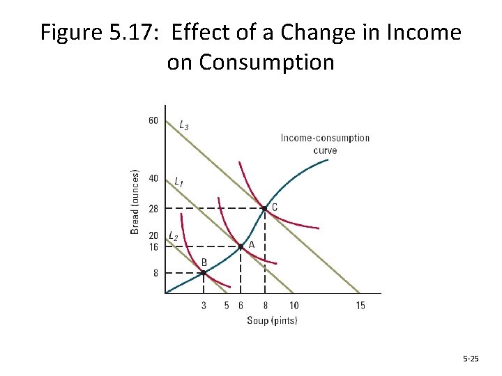
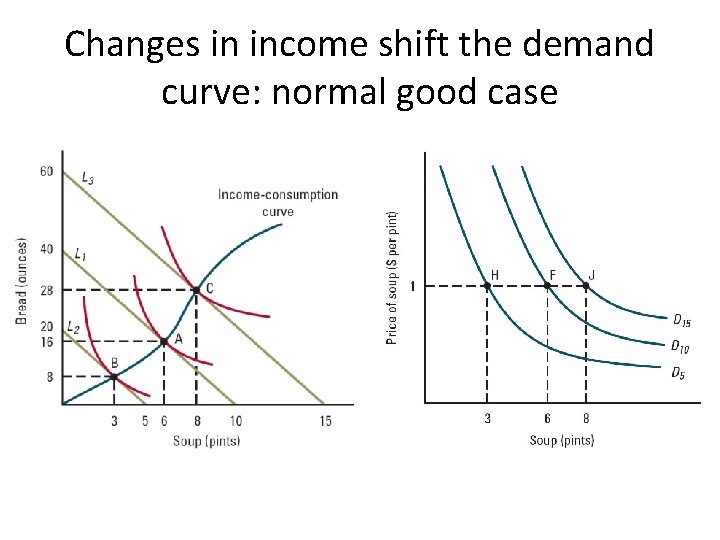
Figure 5. 17: Effect of a Change in Income on Consumption 5 -25

Normal vs. Inferior Goods • If a good is normal, an increase in income raises the amount that is consumed • If a good is inferior, an increase in income decreases the amount that is consumed • Consumption of many goods falls as income rises because people shift toward higher-quality products that fill similar needs – Examples: replace posters with art reproductions, margarine with butter 5 -26

Changes in income shift the demand curve: normal good case

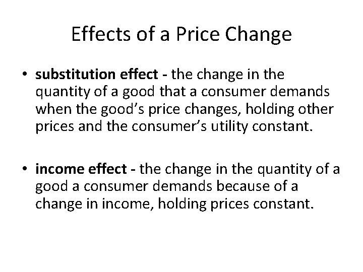
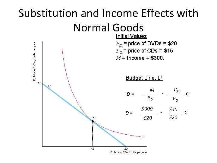
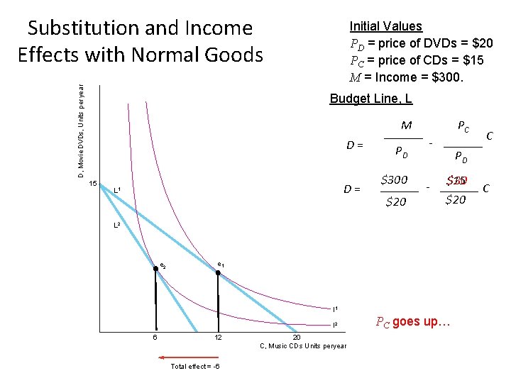
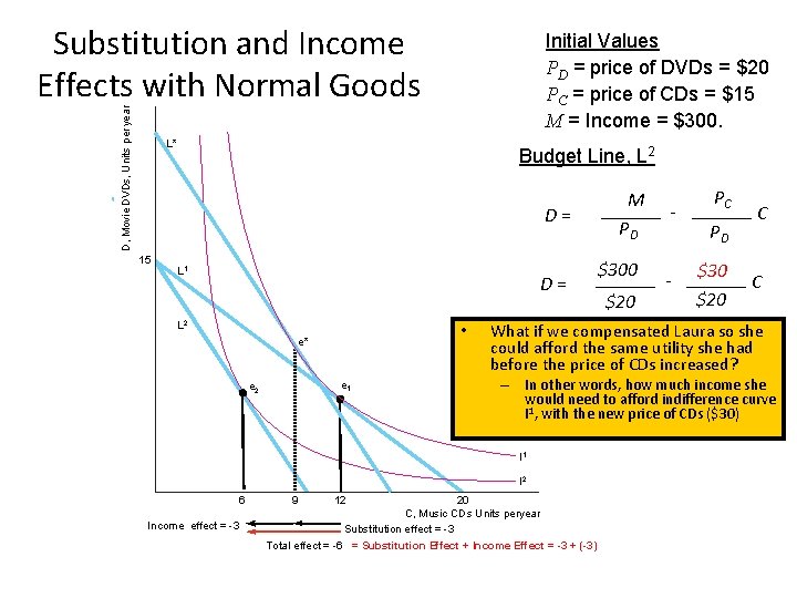
Effects of a Price Change • substitution effect - the change in the quantity of a good that a consumer demands when the good’s price changes, holding other prices and the consumer’s utility constant. • income effect - the change in the quantity of a good a consumer demands because of a change in income, holding prices constant.

Substitution and Income Effects with Normal Goods D, Movie DVDs, Units per year Initial Values PD = price of DVDs = $20 PC = price of CDs = $15 M = Income = $300. Budget Line, L 1 15 L 1 M PD D= e 1 D= $300 $20 I 1 12 20 C, Music CDs Units peryear - PC PD $15 $20 C C

D, Movie DVDs, Units per year Substitution and Income Effects with Normal Goods Initial Values PD = price of DVDs = $20 PC = price of CDs = $15 M = Income = $300. Budget Line, L M D= 15 D= L 1 PD $300 $20 PC - PD $15 $30 $20 L 2 e 1 I 2 6 12 Total effect = -6 20 C, Music CDs Units peryear C PC goes up… C

D, Movie DVDs, Units per year Substitution and Income Effects with Normal Goods Initial Values PD = price of DVDs = $20 PC = price of CDs = $15 M = Income = $300. L* Budget Line, L 2 D= 15 L 1 D= L 2 • e* e 1 e 2 Income effect = -3 12 $20 - PD $30 $20 C C – In other words, how much income she would need to afford indifference curve I 1, with the new price of CDs ($30) I 2 9 $300 - PC What if we compensated Laura so she could afford the same utility she had before the price of CDs increased? I 1 6 M PD 20 C, Music CDs Units peryear Substitution effect = -3 Total effect = -6 = Substitution Effect + Income Effect = -3 + (-3)

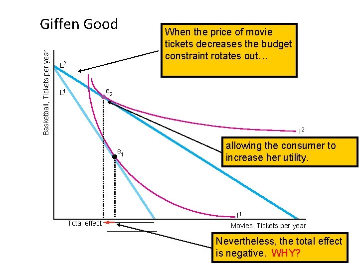
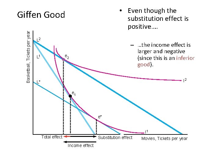
Basketball, Tickets per year Giffen Good L 2 When the price of movie tickets decreases the budget constraint rotates out… e 2 L 1 I 2 e 1 Total effect allowing the consumer to increase her utility. I 1 Movies, Tickets per year Nevertheless, the total effect is negative. WHY?

• Even though the substitution effect is positive…. Basketball, Tickets per year Giffen Good L 2 – …the income effect is larger and negative (since this is an inferior good). e 2 L 1 I 2 L* e 1 e* Total effect Substitution effect Income effect I 1 Movies, Tickets per year

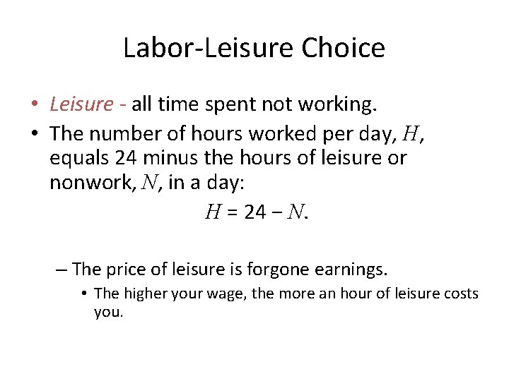
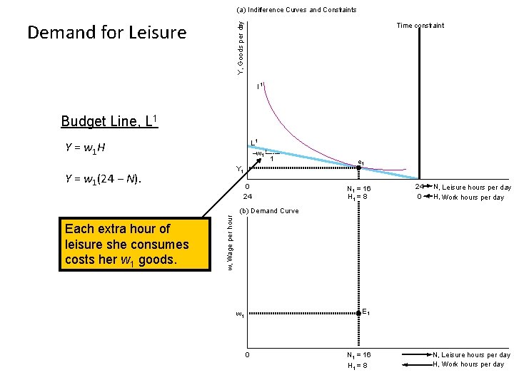
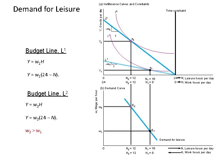
Labor-Leisure Choice • Leisure - all time spent not working. • The number of hours worked per day, H, equals 24 minus the hours of leisure or nonwork, N, in a day: H = 24 − N. – The price of leisure is forgone earnings. • The higher your wage, the more an hour of leisure costs you.

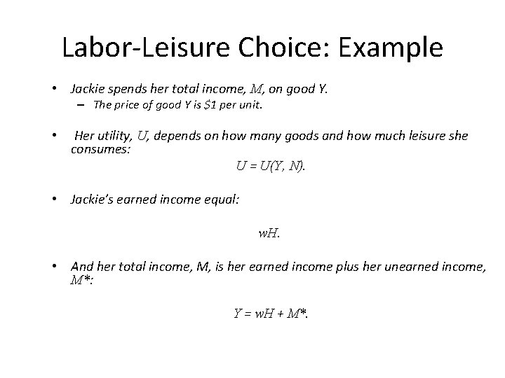
Labor-Leisure Choice: Example • Jackie spends her total income, M, on good Y. – The price of good Y is $1 per unit. • Her utility, U, depends on how many goods and how much leisure she consumes: U = U(Y, N). • Jackie’s earned income equal: w. H. • And her total income, M, is her earned income plus her unearned income, M*: Y = w. H + M*.

(a) Indifference Curves and Constraints Y, Goods per day Demand for Leisure Time constraint I 1 Budget Line, L 1 –w 1 Y = w 1 H 1 Y = w 1(24 − N). 0 24 e 1 N 1 = 16 H 1 = 8 24 0 N, Leisure hours per day H, Work hours per day Each extra hour of leisure she consumes costs her w 1 goods. w, Wage per hour (b) Demand Curve E 1 w 1 0 N 1 = 16 H 1 = 8 N, Leisure hours per day H, Work hours per day

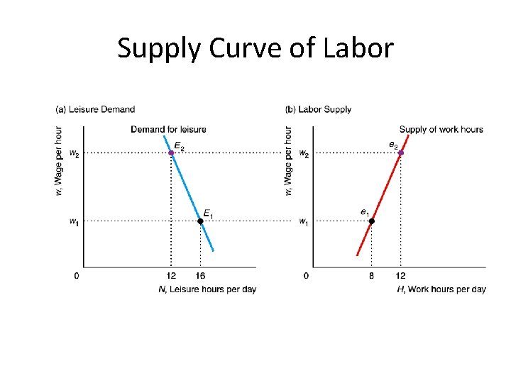
(a) Indifference Curves and Constraints Y, Goods per day Demand for Leisure Time constraint I 2 L 2 –w 2 1 I 1 Y 2 e 2 Budget Line, L 1 –w 1 Y = w 1 H 1 e 1 Y = w 1(24 − N). 0 24 N 2 = 12 H 2 = 12 N 1 = 16 H 1 = 8 24 0 N, Leisure hours per day H, Work hours per day Budget Line, L 2 Y = w 2 H w, Wage per hour (b) Demand Curve E 2 w 2 Y = w 2(24 − N). w 2 > w 1 E 1 w 1 Demand for leisure 0 N 2 = 12 H 2 = 12 N 1 = 16 H 1 = 8 N, Leisure hours per day H, Work hours per day

Supply Curve of Labor

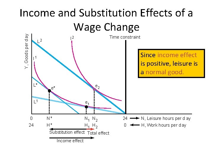
Y, Goods per d ay Income and Substitution Effects of a Wage Change Time constraint I 2 L 2 Since income effect is positive, leisure is a normal good. I 1 L* e 2 e* L 1 e 1 0 N* N 1 N 2 24 N, Leisure hours per d ay 24 H* H 1 H 2 0 H, Work hours per d ay Substitution effect Total effect Income effect

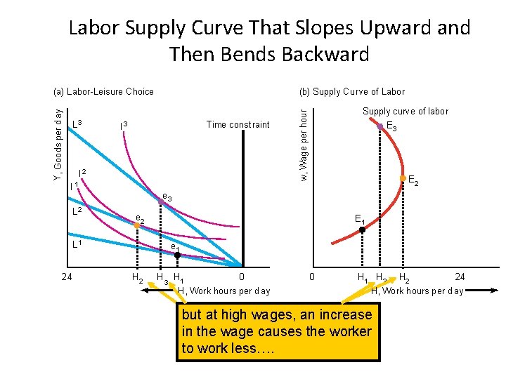
Labor Supply Curve That Slopes Upward and Then Bends Backward L 3 (b) Supply Curve of Labor Time const raint I 3 I 2 I 1 L 2 E 3 E 2 e 3 e 2 E 1 L 1 24 Supply curve of labor w, Wage per hour Y, Goods per d ay (a) Labor-Leisure Choice e 1 H 2 H 3 H 1 0 H, Work hours per d ay 0 H 1 H 3 H 2 24 H, Work hours per d ay butlow At at high wages, an increase in the wage causes the worker to work to less…. work more….

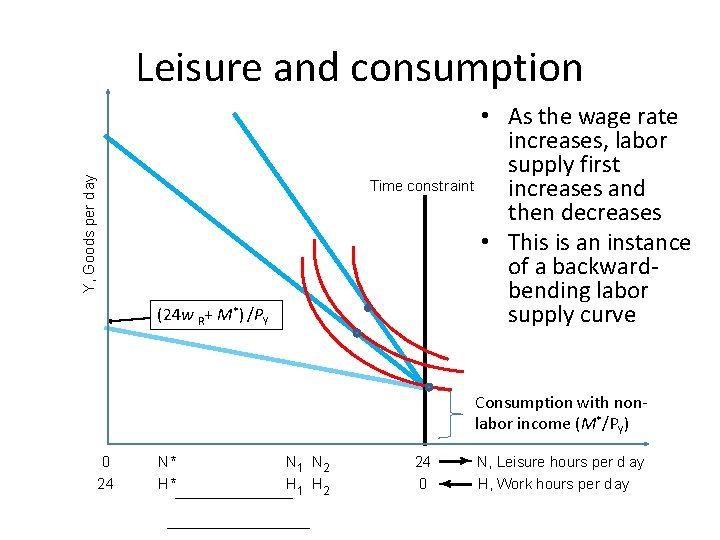
Why leisure is different • When the price of apples goes up, – the substitution effect reduces the consumption of apples, and – Moreover, the consumer’s income decreases in terms of purchasing power. This too reduces the consumption of apples, assuming apples are a normal good • When the wage rate (w), which is also the price of leisure, goes up, the substitution effect works as in the apples example and reduces leisure • But, the higher wage implies not a decrease but an increase in income. This increases leisure, assuming leisure is a normal good • So, although an increase in the price of apples should reasonably be expected to reduce the consumption of apples, an increase in the price of leisure should not be expected to reduce the consumption of leisure • That is, a backward bending labor supply should by no means be considered a freak phenomenon

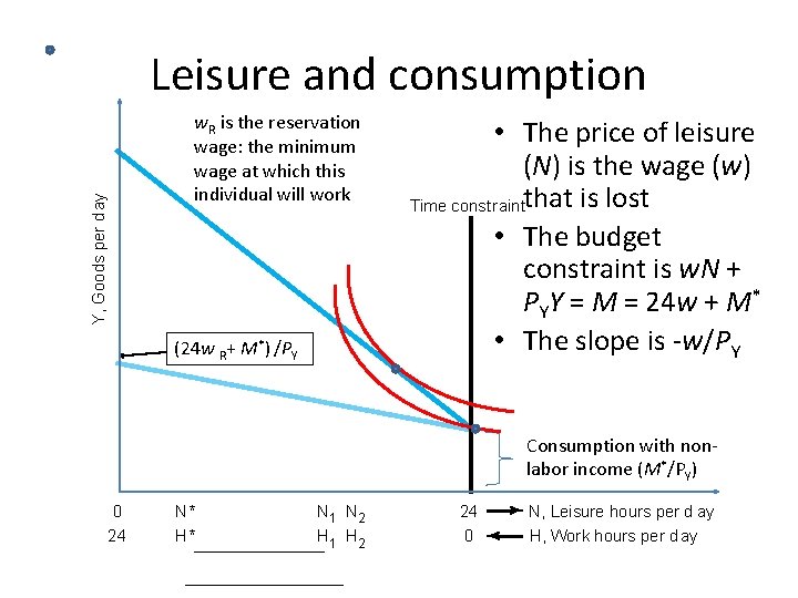
Leisure and consumption Y, Goods per d ay w. R is the reservation wage: the minimum wage at which this individual will work (24 w R+ M*) /PY • The price of leisure (N) is the wage (w) Time constraintthat is lost • The budget constraint is w. N + PYY = M = 24 w + M* • The slope is -w/PY Consumption with nonlabor income (M*/PY) 0 N* N 1 N 2 24 N, Leisure hours per d ay 24 H* H 1 H 2 0 H, Work hours per d ay

Leisure and consumption Y, Goods per d ay • As the wage rate increases, labor supply first Time constraint increases and then decreases • This is an instance of a backwardbending labor supply curve (24 w R+ M*) /PY Consumption with nonlabor income (M*/PY) 0 N* N 1 N 2 24 N, Leisure hours per d ay 24 H* H 1 H 2 0 H, Work hours per d ay