RATIONAL CONSUMER CHOICE Drawing on Chapter 3 Graphics

RATIONAL CONSUMER CHOICE

Drawing on Chapter 3 Graphics copyright © 2010 The Mc. Graw-Hill Companies, Inc. All rights reserved.

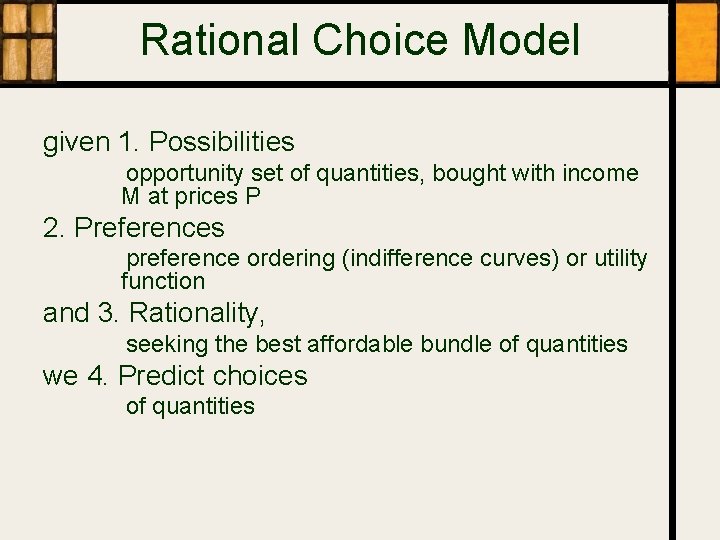
Rational Choice Model given 1. Possibilities opportunity set of quantities, bought with income M at prices P 2. Preferences preference ordering (indifference curves) or utility function and 3. Rationality, seeking the best affordable bundle of quantities we 4. Predict choices of quantities

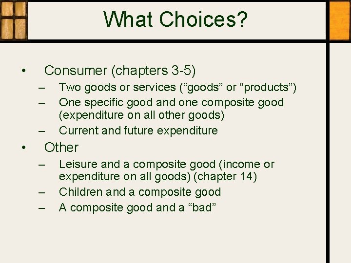
What Choices? • Consumer (chapters 3 -5) – – – • Two goods or services (“goods” or “products”) One specific good and one composite good (expenditure on all other goods) Current and future expenditure Other – – – Leisure and a composite good (income or expenditure on all goods) (chapter 14) Children and a composite good A composite good and a “bad”

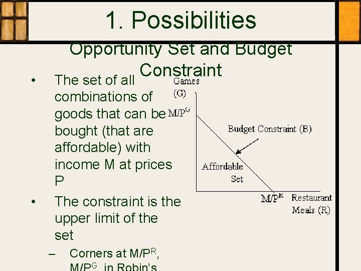
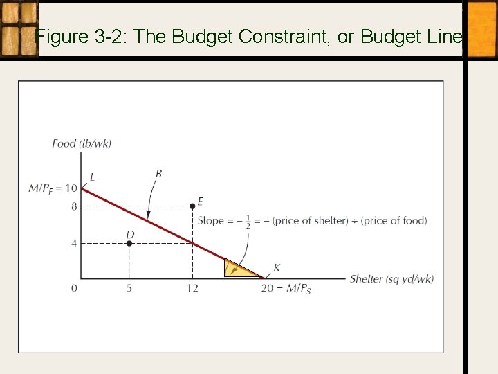
1. Possibilities • • Opportunity Set and Budget Constraint The set of all combinations of goods that can be bought (that are affordable) with income M at prices P The constraint is the upper limit of the set – Corners at M/PR, G

Figure 3 -2: The Budget Constraint, or Budget Line

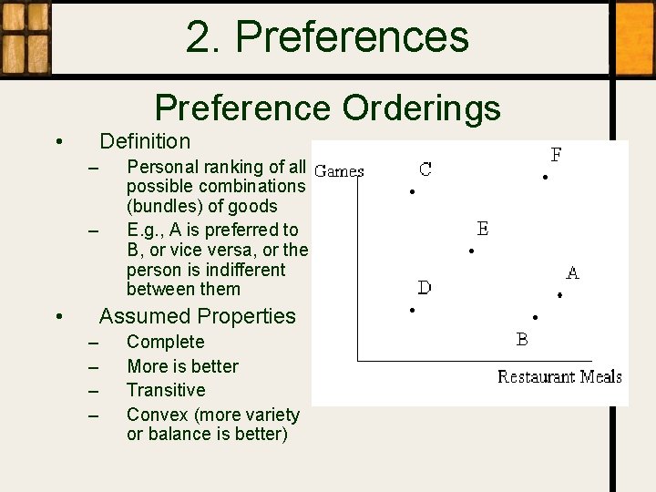
2. Preferences Preference Orderings • Definition – – • Personal ranking of all possible combinations (bundles) of goods E. g. , A is preferred to B, or vice versa, or the person is indifferent between them Assumed Properties – – Complete More is better Transitive Convex (more variety or balance is better)

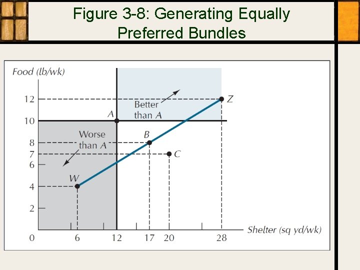
Figure 3 -8: Generating Equally Preferred Bundles

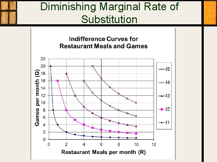
Indifference Curves • Definition – – • A set of equally preferred bundles of goods i. e. , the person is indifferent between them Implied Properties – – Every bundle is on one Negative slope Cannot cross Diminishing |slope|

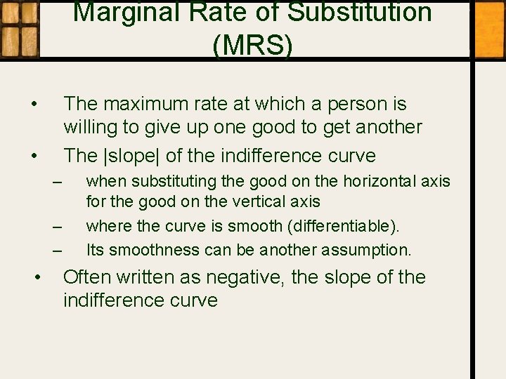
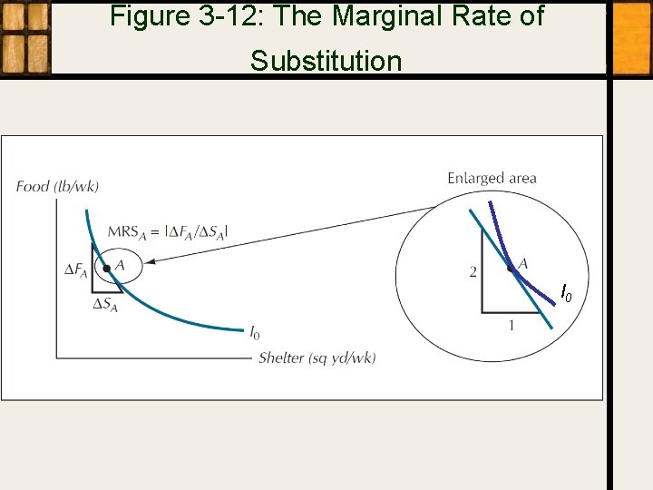
Marginal Rate of Substitution (MRS) • The maximum rate at which a person is willing to give up one good to get another The |slope| of the indifference curve • – – – • when substituting the good on the horizontal axis for the good on the vertical axis where the curve is smooth (differentiable). Its smoothness can be another assumption. Often written as negative, the slope of the indifference curve

Diminishing Marginal Rate of Substitution

Figure 3 -12: The Marginal Rate of Substitution I 0

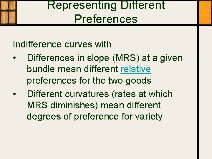
Representing Different Preferences Indifference curves with • Differences in slope (MRS) at a given bundle mean different relative preferences for the two goods • Different curvatures (rates at which MRS diminishes) mean different degrees of preference for variety

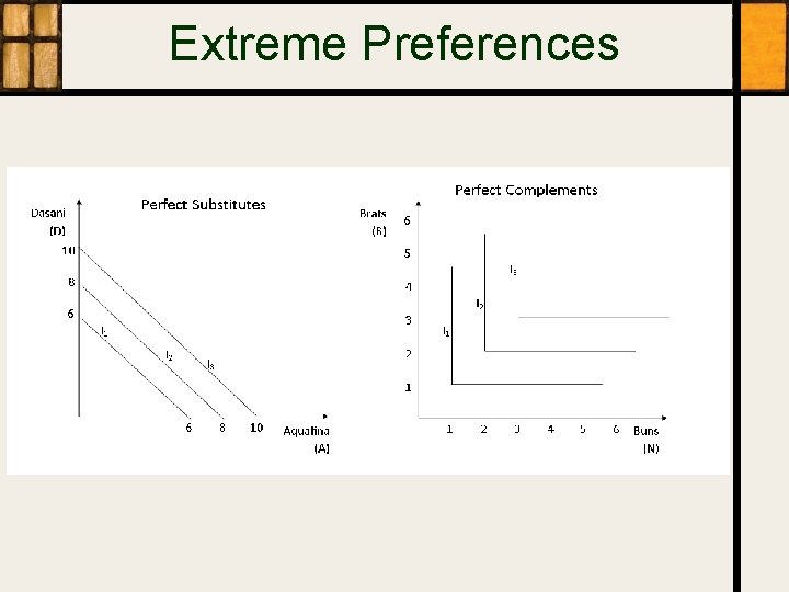
Extreme Preferences

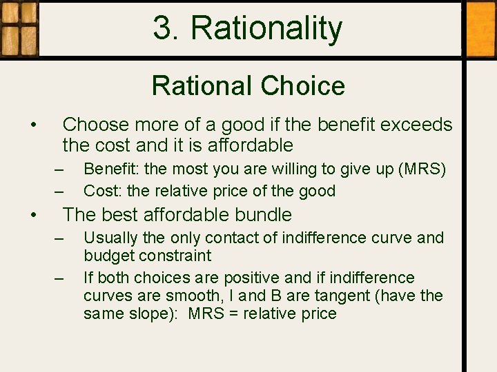
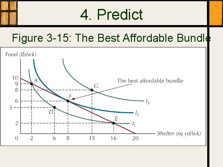
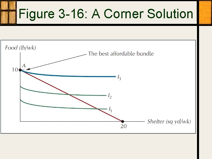
3. Rationality Rational Choice • Choose more of a good if the benefit exceeds the cost and it is affordable – – • Benefit: the most you are willing to give up (MRS) Cost: the relative price of the good The best affordable bundle – – Usually the only contact of indifference curve and budget constraint If both choices are positive and if indifference curves are smooth, I and B are tangent (have the same slope): MRS = relative price

4. Predict Figure 3 -15: The Best Affordable Bundle

Figure 3 -16: A Corner Solution

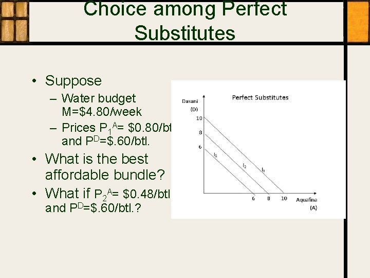
Choice among Perfect Substitutes • Suppose – Water budget M=$4. 80/week – Prices P 1 A= $0. 80/btl. and PD=$. 60/btl. • What is the best affordable bundle? • What if P 2 A= $0. 48/btl. and PD=$. 60/btl. ?

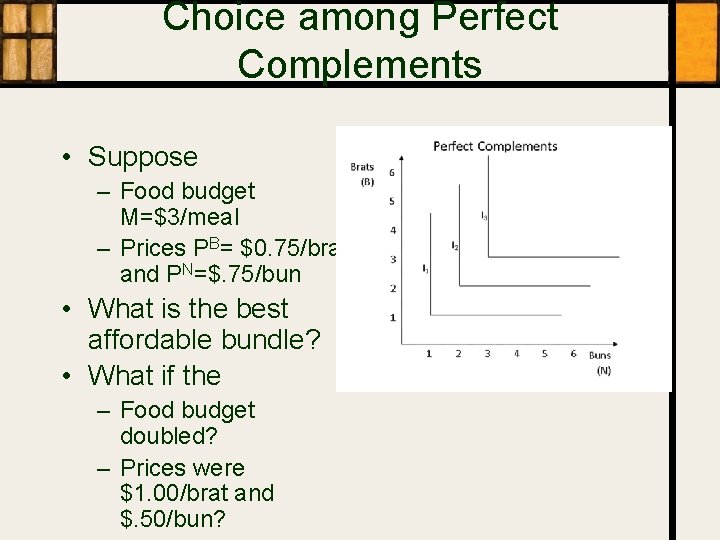
Choice among Perfect Complements • Suppose – Food budget M=$3/meal – Prices PB= $0. 75/brat and PN=$. 75/bun • What is the best affordable bundle? • What if the – Food budget doubled? – Prices were $1. 00/brat and $. 50/bun?

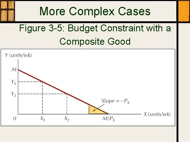
More Complex Cases Figure 3 -5: Budget Constraint with a Composite Good

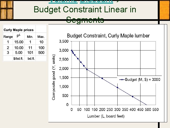
Volume Discount Budget Constraint Linear in Segments

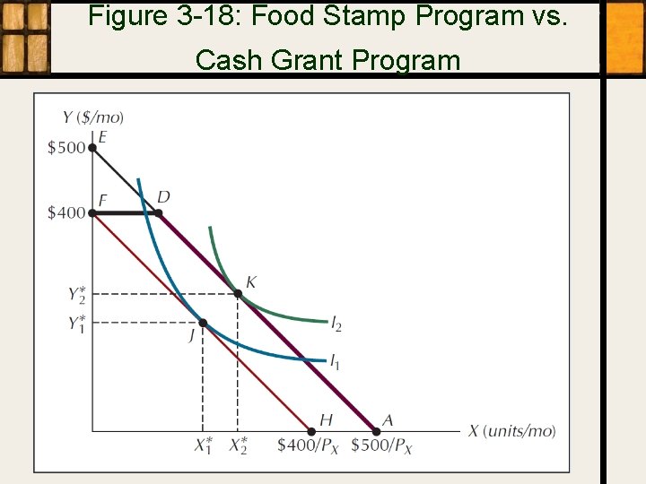
Figure 3 -18: Food Stamp Program vs. Cash Grant Program

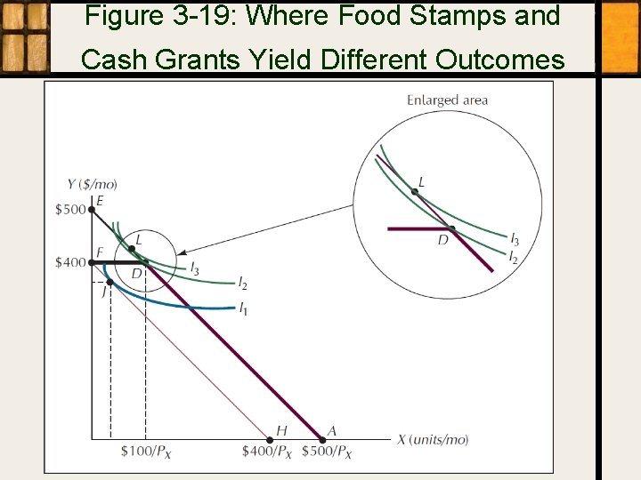
Figure 3 -19: Where Food Stamps and Cash Grants Yield Different Outcomes

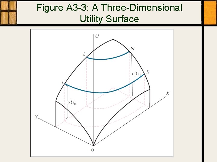
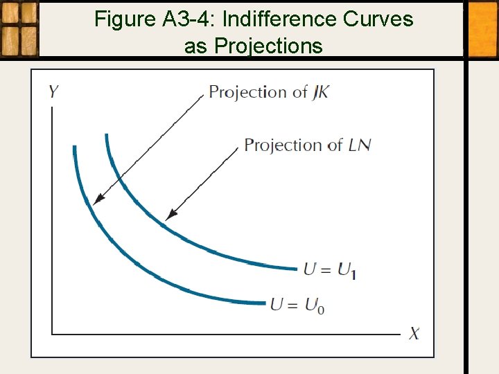
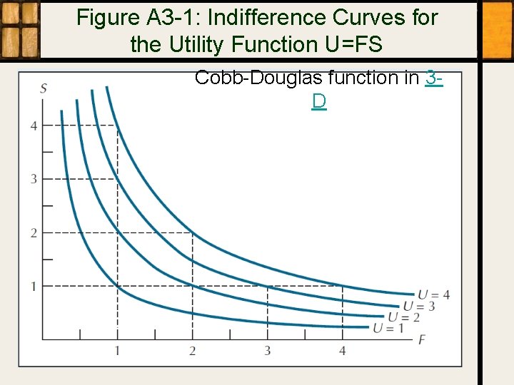
2. Preferences (again) Utility Functions • • Assign a number (indexing utility or satisfaction) to each bundle of goods Assume positive but diminishing marginal utilities (slopes relative to each good’s quantity) Measure utility cardinally, but are better interpreted ordinally Imply indifference curves, each showing bundles providing a given level of utility

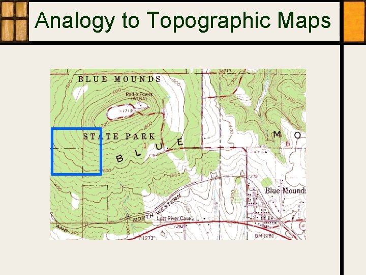
Analogy to Topographic Maps

Figure A 3 -3: A Three-Dimensional Utility Surface

Figure A 3 -4: Indifference Curves as Projections

Figure A 3 -1: Indifference Curves for the Utility Function U=FS Cobb-Douglas function in 3 D

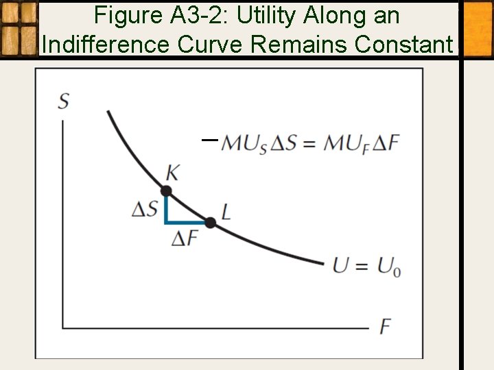
Figure A 3 -2: Utility Along an Indifference Curve Remains Constant

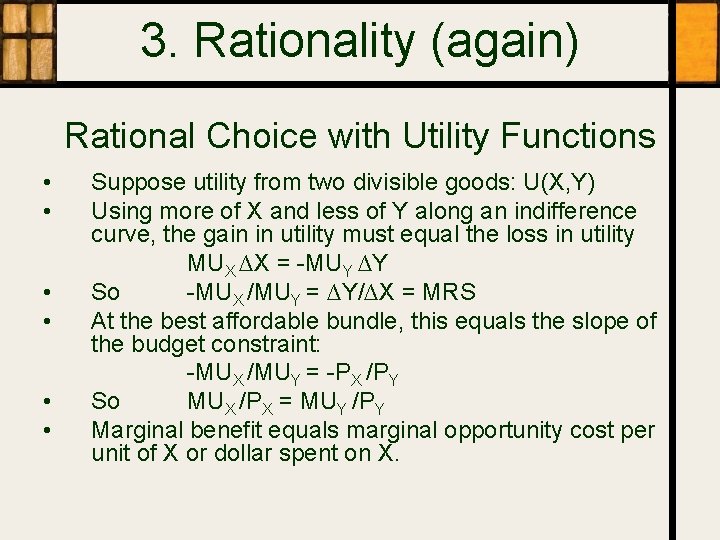
3. Rationality (again) Rational Choice with Utility Functions • • • Suppose utility from two divisible goods: U(X, Y) Using more of X and less of Y along an indifference curve, the gain in utility must equal the loss in utility MUX ∆X = -MUY ∆Y So -MUX /MUY = ∆Y/∆X = MRS At the best affordable bundle, this equals the slope of the budget constraint: -MUX /MUY = -PX /PY So MUX /PX = MUY /PY Marginal benefit equals marginal opportunity cost per unit of X or dollar spent on X.

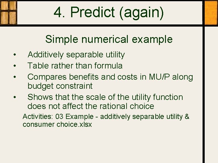
4. Predict (again) Simple numerical example • • Additively separable utility Table rather than formula Compares benefits and costs in MU/P along budget constraint Shows that the scale of the utility function does not affect the rational choice Activities: 03 Example - additively separable utility & consumer choice. xlsx

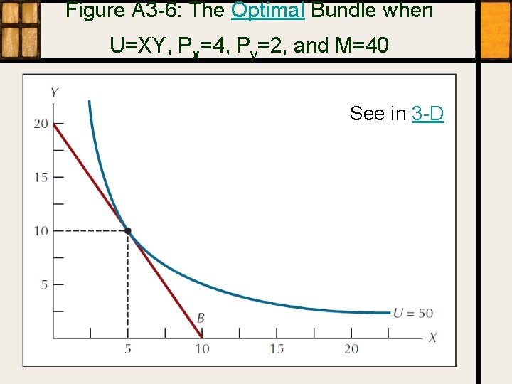
Figure A 3 -6: The Optimal Bundle when U=XY, Px=4, Py=2, and M=40 See in 3 -D

More Examples of Utility Functions Relatively simple, with assumed properties Activities: 03 Examples - utility functions. xlsx

Review • • Predict Rational choice of most Preferred Possibility. Adapts to different Possibilities and Preferences, not to non-rational choice. – – Ordinal ranking is less restrictive. Utility functions are mathematically convenient, and not misleading if interpreted ordinally.